Repository of Reproducible Computations

Free Statistics

of Irreproducible Research!

Author's title

Author

*The author of this computation has been verified*

R Software Module

rwasp_autocorrelation.wasp

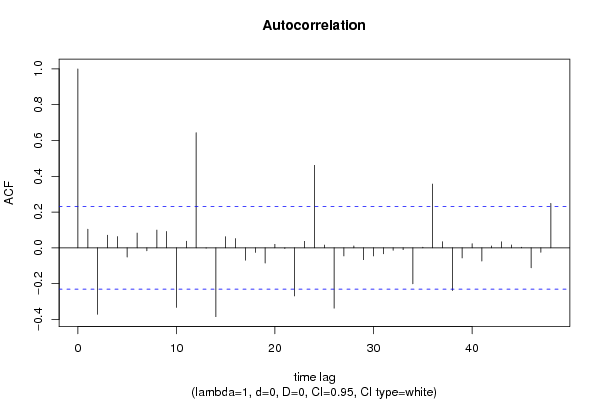
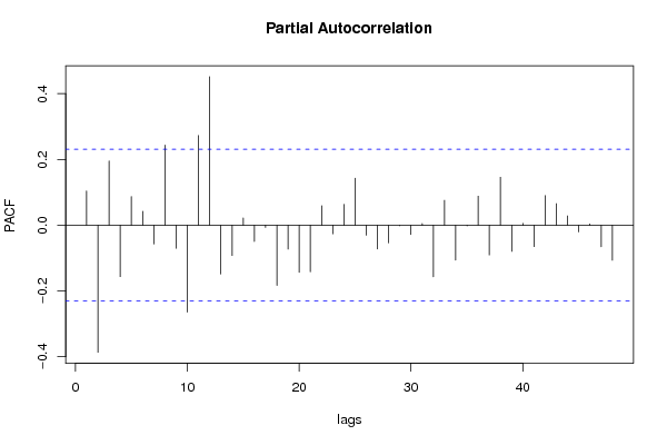
Title produced by software

(Partial) Autocorrelation Function

Date of computation

Tue, 14 Dec 2010 10:11:32 +0000

Cite this page as follows

Statistical Computations at FreeStatistics.org, Office for Research Development and Education, URL https://freestatistics.org/blog/index.php?v=date/2010/Dec/14/t12923214058xoucq41z2yl5sv.htm/, Retrieved Thu, 02 May 2024 20:07:32 +0000

Statistical Computations at FreeStatistics.org, Office for Research Development and Education, URL https://freestatistics.org/blog/index.php?pk=109346, Retrieved Thu, 02 May 2024 20:07:32 +0000

QR Codes:

Paste this QR Code to cite your computation.

Original text written by user:

IsPrivate?

No (this computation is public)

User-defined keywords

Estimated Impact

142

Family? (F = Feedback message, R = changed R code, M = changed R Module, P = changed Parameters, D = changed Data)

-     [(Partial) Autocorrelation Function] [Faillissementen V...] [2010-12-14 08:51:21] [13c73ac943380855a1c72833078e44d2]
-   P   [(Partial) Autocorrelation Function] [Faillissementen V...] [2010-12-14 09:09:28] [13c73ac943380855a1c72833078e44d2]
- RMP     [Spectral Analysis] [Faillissementen V...] [2010-12-14 09:27:52] [13c73ac943380855a1c72833078e44d2]
- RMPD        [(Partial) Autocorrelation Function] [Faillissementen W...] [2010-12-14 10:11:32] [9003764b6a75599accb6eea9154ba195] [Current]
-               [(Partial) Autocorrelation Function] [Faillissementen W...] [2010-12-14 10:14:14] [049b50ae610f671f7417ed8e2d1295c1] 
- RM            [Spectral Analysis] [Faillissementen W...] [2010-12-14 10:17:19] [049b50ae610f671f7417ed8e2d1295c1] 
-                 [Spectral Analysis] [Faillissementen W...] [2010-12-14 10:20:03] [049b50ae610f671f7417ed8e2d1295c1] 
- RM              [Variance Reduction Matrix] [Faillissementen W...] [2010-12-14 10:23:17] [049b50ae610f671f7417ed8e2d1295c1] 
- RM              [Standard Deviation-Mean Plot] [Faillissementen W...] [2010-12-14 10:34:22] [049b50ae610f671f7417ed8e2d1295c1] 
- RM              [ARIMA Backward Selection] [Faillissementen W...] [2010-12-14 10:38:24] [049b50ae610f671f7417ed8e2d1295c1] 
-   PD              [ARIMA Backward Selection] [] [2010-12-17 10:29:12] [13c73ac943380855a1c72833078e44d2] 
- RM              [ARIMA Forecasting] [Faillissementen W...] [2010-12-14 10:41:25] [049b50ae610f671f7417ed8e2d1295c1] 
- RM D            [(Partial) Autocorrelation Function] [Faillissementen B...] [2010-12-14 10:47:49] [3074aa973ede76ac75d398946b01602f] 
-                   [(Partial) Autocorrelation Function] [Faillissementen B...] [2010-12-14 10:50:13] [3074aa973ede76ac75d398946b01602f] 
-                   [(Partial) Autocorrelation Function] [Faillissementen B...] [2010-12-14 10:53:33] [3074aa973ede76ac75d398946b01602f] 

Feedback Forum

Post a new message

Dataseries X:

Download CSV

Histogram

Boxplots

Summary of computational transaction
Raw Input	view raw input (R code)
Raw Output	view raw output of R engine
Computing time	1 seconds
R Server	'Gwilym Jenkins' @ 72.249.127.135

\begin{tabular}{lllllllll}
\hline
Summary of computational transaction \tabularnewline
Raw Input & view raw input (R code)  \tabularnewline
Raw Output & view raw output of R engine  \tabularnewline
Computing time & 1 seconds \tabularnewline
R Server & 'Gwilym Jenkins' @ 72.249.127.135 \tabularnewline
\hline
\end{tabular}
%Source: https://freestatistics.org/blog/index.php?pk=109346&T=0

[TABLE]
[ROW][C]Summary of computational transaction[/C][/ROW]
[ROW][C]Raw Input[/C][C]view raw input (R code) [/C][/ROW]
[ROW][C]Raw Output[/C][C]view raw output of R engine [/C][/ROW]
[ROW][C]Computing time[/C][C]1 seconds[/C][/ROW]
[ROW][C]R Server[/C][C]'Gwilym Jenkins' @ 72.249.127.135[/C][/ROW]
[/TABLE]
Source: https://freestatistics.org/blog/index.php?pk=109346&T=0

Globally Unique Identifier (entire table): ba.freestatistics.org/blog/index.php?pk=109346&T=0

As an alternative you can also use a QR Code:

The GUIDs for individual cells are displayed in the table below:

Summary of computational transaction
Raw Input	view raw input (R code)
Raw Output	view raw output of R engine
Computing time	1 seconds
R Server	'Gwilym Jenkins' @ 72.249.127.135

Autocorrelation Function
Time lag k	ACF(k)	T-STAT	P-value
1	0.104112	0.8834	0.189975
2	-0.37147	-3.152	0.001182
3	0.070607	0.5991	0.275488
4	0.063144	0.5358	0.296875
5	-0.051179	-0.4343	0.332695
6	0.082463	0.6997	0.243178
7	-0.016466	-0.1397	0.444637
8	0.099753	0.8464	0.200059
9	0.091566	0.777	0.219864
10	-0.333	-2.8256	0.003052
11	0.037382	0.3172	0.376005
12	0.643888	5.4636	0
13	-0.001795	-0.0152	0.493946
14	-0.384532	-3.2629	0.000844
15	0.062667	0.5317	0.29827
16	0.051866	0.4401	0.330593
17	-0.068818	-0.5839	0.280542
18	-0.025533	-0.2167	0.414544
19	-0.085032	-0.7215	0.236464
20	0.019948	0.1693	0.433033
21	-0.003805	-0.0323	0.487166
22	-0.268638	-2.2795	0.012802
23	0.036377	0.3087	0.379233
24	0.46156	3.9165	0.000101
25	0.015879	0.1347	0.446598
26	-0.337063	-2.8601	0.002769
27	-0.045491	-0.386	0.350317
28	0.010517	0.0892	0.46457
29	-0.066294	-0.5625	0.287754
30	-0.045519	-0.3862	0.350229
31	-0.033618	-0.2853	0.388132
32	-0.013495	-0.1145	0.454577
33	-0.010193	-0.0865	0.46566
34	-0.200711	-1.7031	0.046433
35	0.00407	0.0345	0.486273
36	0.356838	3.0279	0.001708
37	0.034192	0.2901	0.386276
38	-0.238431	-2.0232	0.023385
39	-0.05633	-0.478	0.317058
40	0.023609	0.2003	0.420893
41	-0.074085	-0.6286	0.265791
42	0.01079	0.0916	0.463652
43	0.033676	0.2857	0.387945
44	0.016519	0.1402	0.44446
45	0.003526	0.0299	0.488107
46	-0.111877	-0.9493	0.17282
47	-0.024814	-0.2106	0.416916
48	0.248661	2.11	0.019169

\begin{tabular}{lllllllll}
\hline
Autocorrelation Function \tabularnewline
Time lag k & ACF(k) & T-STAT & P-value \tabularnewline
1 & 0.104112 & 0.8834 & 0.189975 \tabularnewline
2 & -0.37147 & -3.152 & 0.001182 \tabularnewline
3 & 0.070607 & 0.5991 & 0.275488 \tabularnewline
4 & 0.063144 & 0.5358 & 0.296875 \tabularnewline
5 & -0.051179 & -0.4343 & 0.332695 \tabularnewline
6 & 0.082463 & 0.6997 & 0.243178 \tabularnewline
7 & -0.016466 & -0.1397 & 0.444637 \tabularnewline
8 & 0.099753 & 0.8464 & 0.200059 \tabularnewline
9 & 0.091566 & 0.777 & 0.219864 \tabularnewline
10 & -0.333 & -2.8256 & 0.003052 \tabularnewline
11 & 0.037382 & 0.3172 & 0.376005 \tabularnewline
12 & 0.643888 & 5.4636 & 0 \tabularnewline
13 & -0.001795 & -0.0152 & 0.493946 \tabularnewline
14 & -0.384532 & -3.2629 & 0.000844 \tabularnewline
15 & 0.062667 & 0.5317 & 0.29827 \tabularnewline
16 & 0.051866 & 0.4401 & 0.330593 \tabularnewline
17 & -0.068818 & -0.5839 & 0.280542 \tabularnewline
18 & -0.025533 & -0.2167 & 0.414544 \tabularnewline
19 & -0.085032 & -0.7215 & 0.236464 \tabularnewline
20 & 0.019948 & 0.1693 & 0.433033 \tabularnewline
21 & -0.003805 & -0.0323 & 0.487166 \tabularnewline
22 & -0.268638 & -2.2795 & 0.012802 \tabularnewline
23 & 0.036377 & 0.3087 & 0.379233 \tabularnewline
24 & 0.46156 & 3.9165 & 0.000101 \tabularnewline
25 & 0.015879 & 0.1347 & 0.446598 \tabularnewline
26 & -0.337063 & -2.8601 & 0.002769 \tabularnewline
27 & -0.045491 & -0.386 & 0.350317 \tabularnewline
28 & 0.010517 & 0.0892 & 0.46457 \tabularnewline
29 & -0.066294 & -0.5625 & 0.287754 \tabularnewline
30 & -0.045519 & -0.3862 & 0.350229 \tabularnewline
31 & -0.033618 & -0.2853 & 0.388132 \tabularnewline
32 & -0.013495 & -0.1145 & 0.454577 \tabularnewline
33 & -0.010193 & -0.0865 & 0.46566 \tabularnewline
34 & -0.200711 & -1.7031 & 0.046433 \tabularnewline
35 & 0.00407 & 0.0345 & 0.486273 \tabularnewline
36 & 0.356838 & 3.0279 & 0.001708 \tabularnewline
37 & 0.034192 & 0.2901 & 0.386276 \tabularnewline
38 & -0.238431 & -2.0232 & 0.023385 \tabularnewline
39 & -0.05633 & -0.478 & 0.317058 \tabularnewline
40 & 0.023609 & 0.2003 & 0.420893 \tabularnewline
41 & -0.074085 & -0.6286 & 0.265791 \tabularnewline
42 & 0.01079 & 0.0916 & 0.463652 \tabularnewline
43 & 0.033676 & 0.2857 & 0.387945 \tabularnewline
44 & 0.016519 & 0.1402 & 0.44446 \tabularnewline
45 & 0.003526 & 0.0299 & 0.488107 \tabularnewline
46 & -0.111877 & -0.9493 & 0.17282 \tabularnewline
47 & -0.024814 & -0.2106 & 0.416916 \tabularnewline
48 & 0.248661 & 2.11 & 0.019169 \tabularnewline
\hline
\end{tabular}
%Source: https://freestatistics.org/blog/index.php?pk=109346&T=1

[TABLE]
[ROW][C]Autocorrelation Function[/C][/ROW]
[ROW][C]Time lag k[/C][C]ACF(k)[/C][C]T-STAT[/C][C]P-value[/C][/ROW]
[ROW][C]1[/C][C]0.104112[/C][C]0.8834[/C][C]0.189975[/C][/ROW]
[ROW][C]2[/C][C]-0.37147[/C][C]-3.152[/C][C]0.001182[/C][/ROW]
[ROW][C]3[/C][C]0.070607[/C][C]0.5991[/C][C]0.275488[/C][/ROW]
[ROW][C]4[/C][C]0.063144[/C][C]0.5358[/C][C]0.296875[/C][/ROW]
[ROW][C]5[/C][C]-0.051179[/C][C]-0.4343[/C][C]0.332695[/C][/ROW]
[ROW][C]6[/C][C]0.082463[/C][C]0.6997[/C][C]0.243178[/C][/ROW]
[ROW][C]7[/C][C]-0.016466[/C][C]-0.1397[/C][C]0.444637[/C][/ROW]
[ROW][C]8[/C][C]0.099753[/C][C]0.8464[/C][C]0.200059[/C][/ROW]
[ROW][C]9[/C][C]0.091566[/C][C]0.777[/C][C]0.219864[/C][/ROW]
[ROW][C]10[/C][C]-0.333[/C][C]-2.8256[/C][C]0.003052[/C][/ROW]
[ROW][C]11[/C][C]0.037382[/C][C]0.3172[/C][C]0.376005[/C][/ROW]
[ROW][C]12[/C][C]0.643888[/C][C]5.4636[/C][C]0[/C][/ROW]
[ROW][C]13[/C][C]-0.001795[/C][C]-0.0152[/C][C]0.493946[/C][/ROW]
[ROW][C]14[/C][C]-0.384532[/C][C]-3.2629[/C][C]0.000844[/C][/ROW]
[ROW][C]15[/C][C]0.062667[/C][C]0.5317[/C][C]0.29827[/C][/ROW]
[ROW][C]16[/C][C]0.051866[/C][C]0.4401[/C][C]0.330593[/C][/ROW]
[ROW][C]17[/C][C]-0.068818[/C][C]-0.5839[/C][C]0.280542[/C][/ROW]
[ROW][C]18[/C][C]-0.025533[/C][C]-0.2167[/C][C]0.414544[/C][/ROW]
[ROW][C]19[/C][C]-0.085032[/C][C]-0.7215[/C][C]0.236464[/C][/ROW]
[ROW][C]20[/C][C]0.019948[/C][C]0.1693[/C][C]0.433033[/C][/ROW]
[ROW][C]21[/C][C]-0.003805[/C][C]-0.0323[/C][C]0.487166[/C][/ROW]
[ROW][C]22[/C][C]-0.268638[/C][C]-2.2795[/C][C]0.012802[/C][/ROW]
[ROW][C]23[/C][C]0.036377[/C][C]0.3087[/C][C]0.379233[/C][/ROW]
[ROW][C]24[/C][C]0.46156[/C][C]3.9165[/C][C]0.000101[/C][/ROW]
[ROW][C]25[/C][C]0.015879[/C][C]0.1347[/C][C]0.446598[/C][/ROW]
[ROW][C]26[/C][C]-0.337063[/C][C]-2.8601[/C][C]0.002769[/C][/ROW]
[ROW][C]27[/C][C]-0.045491[/C][C]-0.386[/C][C]0.350317[/C][/ROW]
[ROW][C]28[/C][C]0.010517[/C][C]0.0892[/C][C]0.46457[/C][/ROW]
[ROW][C]29[/C][C]-0.066294[/C][C]-0.5625[/C][C]0.287754[/C][/ROW]
[ROW][C]30[/C][C]-0.045519[/C][C]-0.3862[/C][C]0.350229[/C][/ROW]
[ROW][C]31[/C][C]-0.033618[/C][C]-0.2853[/C][C]0.388132[/C][/ROW]
[ROW][C]32[/C][C]-0.013495[/C][C]-0.1145[/C][C]0.454577[/C][/ROW]
[ROW][C]33[/C][C]-0.010193[/C][C]-0.0865[/C][C]0.46566[/C][/ROW]
[ROW][C]34[/C][C]-0.200711[/C][C]-1.7031[/C][C]0.046433[/C][/ROW]
[ROW][C]35[/C][C]0.00407[/C][C]0.0345[/C][C]0.486273[/C][/ROW]
[ROW][C]36[/C][C]0.356838[/C][C]3.0279[/C][C]0.001708[/C][/ROW]
[ROW][C]37[/C][C]0.034192[/C][C]0.2901[/C][C]0.386276[/C][/ROW]
[ROW][C]38[/C][C]-0.238431[/C][C]-2.0232[/C][C]0.023385[/C][/ROW]
[ROW][C]39[/C][C]-0.05633[/C][C]-0.478[/C][C]0.317058[/C][/ROW]
[ROW][C]40[/C][C]0.023609[/C][C]0.2003[/C][C]0.420893[/C][/ROW]
[ROW][C]41[/C][C]-0.074085[/C][C]-0.6286[/C][C]0.265791[/C][/ROW]
[ROW][C]42[/C][C]0.01079[/C][C]0.0916[/C][C]0.463652[/C][/ROW]
[ROW][C]43[/C][C]0.033676[/C][C]0.2857[/C][C]0.387945[/C][/ROW]
[ROW][C]44[/C][C]0.016519[/C][C]0.1402[/C][C]0.44446[/C][/ROW]
[ROW][C]45[/C][C]0.003526[/C][C]0.0299[/C][C]0.488107[/C][/ROW]
[ROW][C]46[/C][C]-0.111877[/C][C]-0.9493[/C][C]0.17282[/C][/ROW]
[ROW][C]47[/C][C]-0.024814[/C][C]-0.2106[/C][C]0.416916[/C][/ROW]
[ROW][C]48[/C][C]0.248661[/C][C]2.11[/C][C]0.019169[/C][/ROW]
[/TABLE]
Source: https://freestatistics.org/blog/index.php?pk=109346&T=1

Globally Unique Identifier (entire table): ba.freestatistics.org/blog/index.php?pk=109346&T=1

As an alternative you can also use a QR Code:

The GUIDs for individual cells are displayed in the table below:

Autocorrelation Function
Time lag k	ACF(k)	T-STAT	P-value
1	0.104112	0.8834	0.189975
2	-0.37147	-3.152	0.001182
3	0.070607	0.5991	0.275488
4	0.063144	0.5358	0.296875
5	-0.051179	-0.4343	0.332695
6	0.082463	0.6997	0.243178
7	-0.016466	-0.1397	0.444637
8	0.099753	0.8464	0.200059
9	0.091566	0.777	0.219864
10	-0.333	-2.8256	0.003052
11	0.037382	0.3172	0.376005
12	0.643888	5.4636	0
13	-0.001795	-0.0152	0.493946
14	-0.384532	-3.2629	0.000844
15	0.062667	0.5317	0.29827
16	0.051866	0.4401	0.330593
17	-0.068818	-0.5839	0.280542
18	-0.025533	-0.2167	0.414544
19	-0.085032	-0.7215	0.236464
20	0.019948	0.1693	0.433033
21	-0.003805	-0.0323	0.487166
22	-0.268638	-2.2795	0.012802
23	0.036377	0.3087	0.379233
24	0.46156	3.9165	0.000101
25	0.015879	0.1347	0.446598
26	-0.337063	-2.8601	0.002769
27	-0.045491	-0.386	0.350317
28	0.010517	0.0892	0.46457
29	-0.066294	-0.5625	0.287754
30	-0.045519	-0.3862	0.350229
31	-0.033618	-0.2853	0.388132
32	-0.013495	-0.1145	0.454577
33	-0.010193	-0.0865	0.46566
34	-0.200711	-1.7031	0.046433
35	0.00407	0.0345	0.486273
36	0.356838	3.0279	0.001708
37	0.034192	0.2901	0.386276
38	-0.238431	-2.0232	0.023385
39	-0.05633	-0.478	0.317058
40	0.023609	0.2003	0.420893
41	-0.074085	-0.6286	0.265791
42	0.01079	0.0916	0.463652
43	0.033676	0.2857	0.387945
44	0.016519	0.1402	0.44446
45	0.003526	0.0299	0.488107
46	-0.111877	-0.9493	0.17282
47	-0.024814	-0.2106	0.416916
48	0.248661	2.11	0.019169

Partial Autocorrelation Function
Time lag k	PACF(k)	T-STAT	P-value
1	0.104112	0.8834	0.189975
2	-0.386499	-3.2796	0.000802
3	0.19547	1.6586	0.050772
4	-0.156672	-1.3294	0.093955
5	0.086892	0.7373	0.231667
6	0.042153	0.3577	0.360815
7	-0.057153	-0.485	0.31459
8	0.243671	2.0676	0.021135
9	-0.070291	-0.5964	0.276376
10	-0.264598	-2.2452	0.013914
11	0.272686	2.3138	0.011768
12	0.451554	3.8316	0.000135
13	-0.148435	-1.2595	0.105957
14	-0.09232	-0.7834	0.217992
15	0.021811	0.1851	0.426847
16	-0.04965	-0.4213	0.337398
17	-0.006882	-0.0584	0.476797
18	-0.183317	-1.5555	0.062106
19	-0.072881	-0.6184	0.269126
20	-0.143636	-1.2188	0.11345
21	-0.141825	-1.2034	0.116377
22	0.059253	0.5028	0.308328
23	-0.026446	-0.2244	0.411542
24	0.063432	0.5382	0.296035
25	0.143051	1.2138	0.11439
26	-0.030581	-0.2595	0.398
27	-0.072261	-0.6132	0.270854
28	-0.053693	-0.4556	0.325024
29	-0.001598	-0.0136	0.494611
30	-0.028283	-0.24	0.405511
31	0.005163	0.0438	0.482589
32	-0.157126	-1.3333	0.093324
33	0.075788	0.6431	0.261107
34	-0.106407	-0.9029	0.184796
35	-0.002215	-0.0188	0.492527
36	0.088338	0.7496	0.227977
37	-0.090454	-0.7675	0.222638
38	0.145674	1.2361	0.110222
39	-0.079541	-0.6749	0.250941
40	0.005589	0.0474	0.481154
41	-0.065313	-0.5542	0.29058
42	0.090169	0.7651	0.223354
43	0.06562	0.5568	0.289693
44	0.02821	0.2394	0.40575
45	-0.020523	-0.1741	0.431122
46	0.003727	0.0316	0.487431
47	-0.06583	-0.5586	0.28909
48	-0.106871	-0.9068	0.18376

\begin{tabular}{lllllllll}
\hline
Partial Autocorrelation Function \tabularnewline
Time lag k & PACF(k) & T-STAT & P-value \tabularnewline
1 & 0.104112 & 0.8834 & 0.189975 \tabularnewline
2 & -0.386499 & -3.2796 & 0.000802 \tabularnewline
3 & 0.19547 & 1.6586 & 0.050772 \tabularnewline
4 & -0.156672 & -1.3294 & 0.093955 \tabularnewline
5 & 0.086892 & 0.7373 & 0.231667 \tabularnewline
6 & 0.042153 & 0.3577 & 0.360815 \tabularnewline
7 & -0.057153 & -0.485 & 0.31459 \tabularnewline
8 & 0.243671 & 2.0676 & 0.021135 \tabularnewline
9 & -0.070291 & -0.5964 & 0.276376 \tabularnewline
10 & -0.264598 & -2.2452 & 0.013914 \tabularnewline
11 & 0.272686 & 2.3138 & 0.011768 \tabularnewline
12 & 0.451554 & 3.8316 & 0.000135 \tabularnewline
13 & -0.148435 & -1.2595 & 0.105957 \tabularnewline
14 & -0.09232 & -0.7834 & 0.217992 \tabularnewline
15 & 0.021811 & 0.1851 & 0.426847 \tabularnewline
16 & -0.04965 & -0.4213 & 0.337398 \tabularnewline
17 & -0.006882 & -0.0584 & 0.476797 \tabularnewline
18 & -0.183317 & -1.5555 & 0.062106 \tabularnewline
19 & -0.072881 & -0.6184 & 0.269126 \tabularnewline
20 & -0.143636 & -1.2188 & 0.11345 \tabularnewline
21 & -0.141825 & -1.2034 & 0.116377 \tabularnewline
22 & 0.059253 & 0.5028 & 0.308328 \tabularnewline
23 & -0.026446 & -0.2244 & 0.411542 \tabularnewline
24 & 0.063432 & 0.5382 & 0.296035 \tabularnewline
25 & 0.143051 & 1.2138 & 0.11439 \tabularnewline
26 & -0.030581 & -0.2595 & 0.398 \tabularnewline
27 & -0.072261 & -0.6132 & 0.270854 \tabularnewline
28 & -0.053693 & -0.4556 & 0.325024 \tabularnewline
29 & -0.001598 & -0.0136 & 0.494611 \tabularnewline
30 & -0.028283 & -0.24 & 0.405511 \tabularnewline
31 & 0.005163 & 0.0438 & 0.482589 \tabularnewline
32 & -0.157126 & -1.3333 & 0.093324 \tabularnewline
33 & 0.075788 & 0.6431 & 0.261107 \tabularnewline
34 & -0.106407 & -0.9029 & 0.184796 \tabularnewline
35 & -0.002215 & -0.0188 & 0.492527 \tabularnewline
36 & 0.088338 & 0.7496 & 0.227977 \tabularnewline
37 & -0.090454 & -0.7675 & 0.222638 \tabularnewline
38 & 0.145674 & 1.2361 & 0.110222 \tabularnewline
39 & -0.079541 & -0.6749 & 0.250941 \tabularnewline
40 & 0.005589 & 0.0474 & 0.481154 \tabularnewline
41 & -0.065313 & -0.5542 & 0.29058 \tabularnewline
42 & 0.090169 & 0.7651 & 0.223354 \tabularnewline
43 & 0.06562 & 0.5568 & 0.289693 \tabularnewline
44 & 0.02821 & 0.2394 & 0.40575 \tabularnewline
45 & -0.020523 & -0.1741 & 0.431122 \tabularnewline
46 & 0.003727 & 0.0316 & 0.487431 \tabularnewline
47 & -0.06583 & -0.5586 & 0.28909 \tabularnewline
48 & -0.106871 & -0.9068 & 0.18376 \tabularnewline
\hline
\end{tabular}
%Source: https://freestatistics.org/blog/index.php?pk=109346&T=2

[TABLE]
[ROW][C]Partial Autocorrelation Function[/C][/ROW]
[ROW][C]Time lag k[/C][C]PACF(k)[/C][C]T-STAT[/C][C]P-value[/C][/ROW]
[ROW][C]1[/C][C]0.104112[/C][C]0.8834[/C][C]0.189975[/C][/ROW]
[ROW][C]2[/C][C]-0.386499[/C][C]-3.2796[/C][C]0.000802[/C][/ROW]
[ROW][C]3[/C][C]0.19547[/C][C]1.6586[/C][C]0.050772[/C][/ROW]
[ROW][C]4[/C][C]-0.156672[/C][C]-1.3294[/C][C]0.093955[/C][/ROW]
[ROW][C]5[/C][C]0.086892[/C][C]0.7373[/C][C]0.231667[/C][/ROW]
[ROW][C]6[/C][C]0.042153[/C][C]0.3577[/C][C]0.360815[/C][/ROW]
[ROW][C]7[/C][C]-0.057153[/C][C]-0.485[/C][C]0.31459[/C][/ROW]
[ROW][C]8[/C][C]0.243671[/C][C]2.0676[/C][C]0.021135[/C][/ROW]
[ROW][C]9[/C][C]-0.070291[/C][C]-0.5964[/C][C]0.276376[/C][/ROW]
[ROW][C]10[/C][C]-0.264598[/C][C]-2.2452[/C][C]0.013914[/C][/ROW]
[ROW][C]11[/C][C]0.272686[/C][C]2.3138[/C][C]0.011768[/C][/ROW]
[ROW][C]12[/C][C]0.451554[/C][C]3.8316[/C][C]0.000135[/C][/ROW]
[ROW][C]13[/C][C]-0.148435[/C][C]-1.2595[/C][C]0.105957[/C][/ROW]
[ROW][C]14[/C][C]-0.09232[/C][C]-0.7834[/C][C]0.217992[/C][/ROW]
[ROW][C]15[/C][C]0.021811[/C][C]0.1851[/C][C]0.426847[/C][/ROW]
[ROW][C]16[/C][C]-0.04965[/C][C]-0.4213[/C][C]0.337398[/C][/ROW]
[ROW][C]17[/C][C]-0.006882[/C][C]-0.0584[/C][C]0.476797[/C][/ROW]
[ROW][C]18[/C][C]-0.183317[/C][C]-1.5555[/C][C]0.062106[/C][/ROW]
[ROW][C]19[/C][C]-0.072881[/C][C]-0.6184[/C][C]0.269126[/C][/ROW]
[ROW][C]20[/C][C]-0.143636[/C][C]-1.2188[/C][C]0.11345[/C][/ROW]
[ROW][C]21[/C][C]-0.141825[/C][C]-1.2034[/C][C]0.116377[/C][/ROW]
[ROW][C]22[/C][C]0.059253[/C][C]0.5028[/C][C]0.308328[/C][/ROW]
[ROW][C]23[/C][C]-0.026446[/C][C]-0.2244[/C][C]0.411542[/C][/ROW]
[ROW][C]24[/C][C]0.063432[/C][C]0.5382[/C][C]0.296035[/C][/ROW]
[ROW][C]25[/C][C]0.143051[/C][C]1.2138[/C][C]0.11439[/C][/ROW]
[ROW][C]26[/C][C]-0.030581[/C][C]-0.2595[/C][C]0.398[/C][/ROW]
[ROW][C]27[/C][C]-0.072261[/C][C]-0.6132[/C][C]0.270854[/C][/ROW]
[ROW][C]28[/C][C]-0.053693[/C][C]-0.4556[/C][C]0.325024[/C][/ROW]
[ROW][C]29[/C][C]-0.001598[/C][C]-0.0136[/C][C]0.494611[/C][/ROW]
[ROW][C]30[/C][C]-0.028283[/C][C]-0.24[/C][C]0.405511[/C][/ROW]
[ROW][C]31[/C][C]0.005163[/C][C]0.0438[/C][C]0.482589[/C][/ROW]
[ROW][C]32[/C][C]-0.157126[/C][C]-1.3333[/C][C]0.093324[/C][/ROW]
[ROW][C]33[/C][C]0.075788[/C][C]0.6431[/C][C]0.261107[/C][/ROW]
[ROW][C]34[/C][C]-0.106407[/C][C]-0.9029[/C][C]0.184796[/C][/ROW]
[ROW][C]35[/C][C]-0.002215[/C][C]-0.0188[/C][C]0.492527[/C][/ROW]
[ROW][C]36[/C][C]0.088338[/C][C]0.7496[/C][C]0.227977[/C][/ROW]
[ROW][C]37[/C][C]-0.090454[/C][C]-0.7675[/C][C]0.222638[/C][/ROW]
[ROW][C]38[/C][C]0.145674[/C][C]1.2361[/C][C]0.110222[/C][/ROW]
[ROW][C]39[/C][C]-0.079541[/C][C]-0.6749[/C][C]0.250941[/C][/ROW]
[ROW][C]40[/C][C]0.005589[/C][C]0.0474[/C][C]0.481154[/C][/ROW]
[ROW][C]41[/C][C]-0.065313[/C][C]-0.5542[/C][C]0.29058[/C][/ROW]
[ROW][C]42[/C][C]0.090169[/C][C]0.7651[/C][C]0.223354[/C][/ROW]
[ROW][C]43[/C][C]0.06562[/C][C]0.5568[/C][C]0.289693[/C][/ROW]
[ROW][C]44[/C][C]0.02821[/C][C]0.2394[/C][C]0.40575[/C][/ROW]
[ROW][C]45[/C][C]-0.020523[/C][C]-0.1741[/C][C]0.431122[/C][/ROW]
[ROW][C]46[/C][C]0.003727[/C][C]0.0316[/C][C]0.487431[/C][/ROW]
[ROW][C]47[/C][C]-0.06583[/C][C]-0.5586[/C][C]0.28909[/C][/ROW]
[ROW][C]48[/C][C]-0.106871[/C][C]-0.9068[/C][C]0.18376[/C][/ROW]
[/TABLE]
Source: https://freestatistics.org/blog/index.php?pk=109346&T=2

Globally Unique Identifier (entire table): ba.freestatistics.org/blog/index.php?pk=109346&T=2

As an alternative you can also use a QR Code:

The GUIDs for individual cells are displayed in the table below:

Partial Autocorrelation Function
Time lag k	PACF(k)	T-STAT	P-value
1	0.104112	0.8834	0.189975
2	-0.386499	-3.2796	0.000802
3	0.19547	1.6586	0.050772
4	-0.156672	-1.3294	0.093955
5	0.086892	0.7373	0.231667
6	0.042153	0.3577	0.360815
7	-0.057153	-0.485	0.31459
8	0.243671	2.0676	0.021135
9	-0.070291	-0.5964	0.276376
10	-0.264598	-2.2452	0.013914
11	0.272686	2.3138	0.011768
12	0.451554	3.8316	0.000135
13	-0.148435	-1.2595	0.105957
14	-0.09232	-0.7834	0.217992
15	0.021811	0.1851	0.426847
16	-0.04965	-0.4213	0.337398
17	-0.006882	-0.0584	0.476797
18	-0.183317	-1.5555	0.062106
19	-0.072881	-0.6184	0.269126
20	-0.143636	-1.2188	0.11345
21	-0.141825	-1.2034	0.116377
22	0.059253	0.5028	0.308328
23	-0.026446	-0.2244	0.411542
24	0.063432	0.5382	0.296035
25	0.143051	1.2138	0.11439
26	-0.030581	-0.2595	0.398
27	-0.072261	-0.6132	0.270854
28	-0.053693	-0.4556	0.325024
29	-0.001598	-0.0136	0.494611
30	-0.028283	-0.24	0.405511
31	0.005163	0.0438	0.482589
32	-0.157126	-1.3333	0.093324
33	0.075788	0.6431	0.261107
34	-0.106407	-0.9029	0.184796
35	-0.002215	-0.0188	0.492527
36	0.088338	0.7496	0.227977
37	-0.090454	-0.7675	0.222638
38	0.145674	1.2361	0.110222
39	-0.079541	-0.6749	0.250941
40	0.005589	0.0474	0.481154
41	-0.065313	-0.5542	0.29058
42	0.090169	0.7651	0.223354
43	0.06562	0.5568	0.289693
44	0.02821	0.2394	0.40575
45	-0.020523	-0.1741	0.431122
46	0.003727	0.0316	0.487431
47	-0.06583	-0.5586	0.28909
48	-0.106871	-0.9068	0.18376

Figure 1

PNG link

Postscript link

PDF link

Figure 2

PNG link

Postscript link

PDF link

Parameters (Session):

par1 = 12 ;

Parameters (R input):

par1 = 48 ; par2 = 1 ; par3 = 0 ; par4 = 0 ; par5 = 12 ; par6 = White Noise ; par7 = 0.95 ;

R code (references can be found in the software module):

if (par1 == 'Default') {
par1 = 10*log10(length(x))
} else {
par1 <- as.numeric(par1)
}
par2 <- as.numeric(par2)
par3 <- as.numeric(par3)
par4 <- as.numeric(par4)
par5 <- as.numeric(par5)
if (par6 == 'White Noise') par6 <- 'white' else par6 <- 'ma'
par7 <- as.numeric(par7)
if (par2 == 0) {
x <- log(x)
} else {
x <- (x ^ par2 - 1) / par2
}
if (par3 > 0) x <- diff(x,lag=1,difference=par3)
if (par4 > 0) x <- diff(x,lag=par5,difference=par4)
bitmap(file='pic1.png')
racf <- acf(x, par1, main='Autocorrelation', xlab='time lag', ylab='ACF', ci.type=par6, ci=par7, sub=paste('(lambda=',par2,', d=',par3,', D=',par4,', CI=', par7, ', CI type=',par6,')',sep=''))
dev.off()
bitmap(file='pic2.png')
rpacf <- pacf(x,par1,main='Partial Autocorrelation',xlab='lags',ylab='PACF')
dev.off()
(myacf <- c(racf$acf))
(mypacf <- c(rpacf$acf))
lengthx <- length(x)
sqrtn <- sqrt(lengthx)
load(file='createtable')
a<-table.start()
a<-table.row.start(a)
a<-table.element(a,'Autocorrelation Function',4,TRUE)
a<-table.row.end(a)
a<-table.row.start(a)
a<-table.element(a,'Time lag k',header=TRUE)
a<-table.element(a,hyperlink('basics.htm','ACF(k)','click here for more information about the Autocorrelation Function'),header=TRUE)
a<-table.element(a,'T-STAT',header=TRUE)
a<-table.element(a,'P-value',header=TRUE)
a<-table.row.end(a)
for (i in 2:(par1+1)) {
a<-table.row.start(a)
a<-table.element(a,i-1,header=TRUE)
a<-table.element(a,round(myacf[i],6))
mytstat <- myacf[i]*sqrtn
a<-table.element(a,round(mytstat,4))
a<-table.element(a,round(1-pt(abs(mytstat),lengthx),6))
a<-table.row.end(a)
}
a<-table.end(a)
table.save(a,file='mytable.tab')
a<-table.start()
a<-table.row.start(a)
a<-table.element(a,'Partial Autocorrelation Function',4,TRUE)
a<-table.row.end(a)
a<-table.row.start(a)
a<-table.element(a,'Time lag k',header=TRUE)
a<-table.element(a,hyperlink('basics.htm','PACF(k)','click here for more information about the Partial Autocorrelation Function'),header=TRUE)
a<-table.element(a,'T-STAT',header=TRUE)
a<-table.element(a,'P-value',header=TRUE)
a<-table.row.end(a)
for (i in 1:par1) {
a<-table.row.start(a)
a<-table.element(a,i,header=TRUE)
a<-table.element(a,round(mypacf[i],6))
mytstat <- mypacf[i]*sqrtn
a<-table.element(a,round(mytstat,4))
a<-table.element(a,round(1-pt(abs(mytstat),lengthx),6))
a<-table.row.end(a)
}
a<-table.end(a)
table.save(a,file='mytable1.tab')

Free Statistics

Description of Statistical Computation

Tree of Dependent Computations

Dataset

Tables (Output of Computation)

Figures (Output of Computation)

Input Parameters & R Code