Repository of Reproducible Computations

Free Statistics

of Irreproducible Research!

Author's title

Author

*The author of this computation has been verified*

R Software Module

rwasp_autocorrelation.wasp

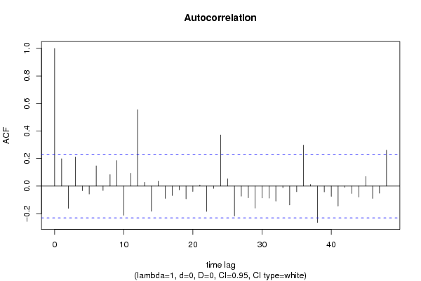
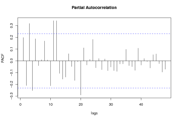
Title produced by software

(Partial) Autocorrelation Function

Date of computation

Tue, 14 Dec 2010 08:51:21 +0000

Cite this page as follows

Statistical Computations at FreeStatistics.org, Office for Research Development and Education, URL https://freestatistics.org/blog/index.php?v=date/2010/Dec/14/t1292316589y9difsppbo8ktxy.htm/, Retrieved Thu, 02 May 2024 17:30:10 +0000

Statistical Computations at FreeStatistics.org, Office for Research Development and Education, URL https://freestatistics.org/blog/index.php?pk=109264, Retrieved Thu, 02 May 2024 17:30:10 +0000

QR Codes:

Paste this QR Code to cite your computation.

Original text written by user:

IsPrivate?

No (this computation is public)

User-defined keywords

Estimated Impact

195

Family? (F = Feedback message, R = changed R code, M = changed R Module, P = changed Parameters, D = changed Data)

-       [(Partial) Autocorrelation Function] [Faillissementen V...] [2010-12-14 08:51:21] [8e16b01a5be2b3f7f3ad6418d9d6fd5b] [Current]
-   P     [(Partial) Autocorrelation Function] [Faillissementen V...] [2010-12-14 09:09:28] [13c73ac943380855a1c72833078e44d2] 
-   P       [(Partial) Autocorrelation Function] [Faillissementen V...] [2010-12-14 09:17:43] [13c73ac943380855a1c72833078e44d2] 
- RMP       [Spectral Analysis] [Faillissementen V...] [2010-12-14 09:27:52] [13c73ac943380855a1c72833078e44d2] 
- RMP       [Spectral Analysis] [Faillissementen V...] [2010-12-14 09:27:52] [13c73ac943380855a1c72833078e44d2] 
- RMP       [Spectral Analysis] [Faillissementen V...] [2010-12-14 09:27:52] [13c73ac943380855a1c72833078e44d2] 
- RMP       [Spectral Analysis] [Faillissementen V...] [2010-12-14 09:27:52] [13c73ac943380855a1c72833078e44d2] 
-   P         [Spectral Analysis] [Faillissementen V...] [2010-12-14 09:35:08] [13c73ac943380855a1c72833078e44d2] 
- RMP         [Standard Deviation-Mean Plot] [Faillissementen V...] [2010-12-14 09:42:21] [13c73ac943380855a1c72833078e44d2] 
- RMP         [ARIMA Backward Selection] [Faillissementen V...] [2010-12-14 09:52:00] [13c73ac943380855a1c72833078e44d2] 
- RMP         [ARIMA Forecasting] [Faillissementen V...] [2010-12-14 10:04:12] [13c73ac943380855a1c72833078e44d2] 
- RMPD        [(Partial) Autocorrelation Function] [Faillissementen W...] [2010-12-14 10:11:32] [049b50ae610f671f7417ed8e2d1295c1] 
-               [(Partial) Autocorrelation Function] [Faillissementen W...] [2010-12-14 10:14:14] [049b50ae610f671f7417ed8e2d1295c1] 
- RM            [Spectral Analysis] [Faillissementen W...] [2010-12-14 10:17:19] [049b50ae610f671f7417ed8e2d1295c1] 
-                 [Spectral Analysis] [Faillissementen W...] [2010-12-14 10:20:03] [049b50ae610f671f7417ed8e2d1295c1] 
- RM              [Variance Reduction Matrix] [Faillissementen W...] [2010-12-14 10:23:17] [049b50ae610f671f7417ed8e2d1295c1] 
- RM              [Standard Deviation-Mean Plot] [Faillissementen W...] [2010-12-14 10:34:22] [049b50ae610f671f7417ed8e2d1295c1] 
- RM              [ARIMA Backward Selection] [Faillissementen W...] [2010-12-14 10:38:24] [049b50ae610f671f7417ed8e2d1295c1] 
-   PD              [ARIMA Backward Selection] [] [2010-12-17 10:29:12] [13c73ac943380855a1c72833078e44d2] 
- RM              [ARIMA Forecasting] [Faillissementen W...] [2010-12-14 10:41:25] [049b50ae610f671f7417ed8e2d1295c1] 
- RM D            [(Partial) Autocorrelation Function] [Faillissementen B...] [2010-12-14 10:47:49] [3074aa973ede76ac75d398946b01602f] 
-                   [(Partial) Autocorrelation Function] [Faillissementen B...] [2010-12-14 10:50:13] [3074aa973ede76ac75d398946b01602f] 
-                   [(Partial) Autocorrelation Function] [Faillissementen B...] [2010-12-14 10:53:33] [3074aa973ede76ac75d398946b01602f] 

Feedback Forum

Post a new message

Dataseries X:

Download CSV

Histogram

Boxplots

Summary of computational transaction
Raw Input	view raw input (R code)
Raw Output	view raw output of R engine
Computing time	29 seconds
R Server	'Gwilym Jenkins' @ 72.249.127.135

\begin{tabular}{lllllllll}
\hline
Summary of computational transaction \tabularnewline
Raw Input & view raw input (R code)  \tabularnewline
Raw Output & view raw output of R engine  \tabularnewline
Computing time & 29 seconds \tabularnewline
R Server & 'Gwilym Jenkins' @ 72.249.127.135 \tabularnewline
\hline
\end{tabular}
%Source: https://freestatistics.org/blog/index.php?pk=109264&T=0

[TABLE]
[ROW][C]Summary of computational transaction[/C][/ROW]
[ROW][C]Raw Input[/C][C]view raw input (R code) [/C][/ROW]
[ROW][C]Raw Output[/C][C]view raw output of R engine [/C][/ROW]
[ROW][C]Computing time[/C][C]29 seconds[/C][/ROW]
[ROW][C]R Server[/C][C]'Gwilym Jenkins' @ 72.249.127.135[/C][/ROW]
[/TABLE]
Source: https://freestatistics.org/blog/index.php?pk=109264&T=0

Globally Unique Identifier (entire table): ba.freestatistics.org/blog/index.php?pk=109264&T=0

As an alternative you can also use a QR Code:

The GUIDs for individual cells are displayed in the table below:

Summary of computational transaction
Raw Input	view raw input (R code)
Raw Output	view raw output of R engine
Computing time	29 seconds
R Server	'Gwilym Jenkins' @ 72.249.127.135

Autocorrelation Function
Time lag k	ACF(k)	T-STAT	P-value
1	0.198742	1.6864	0.048026
2	-0.162152	-1.3759	0.086558
3	0.211306	1.793	0.038587
4	-0.034009	-0.2886	0.386866
5	-0.058207	-0.4939	0.311438
6	0.146935	1.2468	0.108259
7	-0.032286	-0.274	0.392452
8	0.082995	0.7042	0.241779
9	0.185444	1.5735	0.059988
10	-0.212378	-1.8021	0.037859
11	0.09329	0.7916	0.2156
12	0.555231	4.7113	6e-06
13	0.027633	0.2345	0.407643
14	-0.183208	-1.5546	0.062216
15	0.034997	0.297	0.383677
16	-0.090139	-0.7649	0.223429
17	-0.068743	-0.5833	0.280756
18	-0.027829	-0.2361	0.407
19	-0.093308	-0.7917	0.215554
20	-0.039437	-0.3346	0.369437
21	0.007861	0.0667	0.473502
22	-0.184306	-1.5639	0.061114
23	-0.016781	-0.1424	0.443584
24	0.371231	3.15	0.001189
25	0.05259	0.4462	0.328381
26	-0.217443	-1.8451	0.03457
27	-0.074084	-0.6286	0.265793
28	-0.0853	-0.7238	0.235768
29	-0.159719	-1.3553	0.089785
30	-0.086797	-0.7365	0.231911
31	-0.088073	-0.7473	0.228652
32	-0.109462	-0.9288	0.178044
33	-0.012413	-0.1053	0.458205
34	-0.137987	-1.1709	0.122757
35	-0.041594	-0.3529	0.362583
36	0.297195	2.5218	0.006945
37	0.011653	0.0989	0.460756
38	-0.264505	-2.2444	0.013941
39	-0.042386	-0.3597	0.360079
40	-0.075224	-0.6383	0.262652
41	-0.145331	-1.2332	0.110761
42	-0.009724	-0.0825	0.467234
43	-0.053904	-0.4574	0.324383
44	-0.08028	-0.6812	0.248966
45	0.069951	0.5936	0.277335
46	-0.089813	-0.7621	0.224248
47	-0.052288	-0.4437	0.329304
48	0.261046	2.215	0.01496

\begin{tabular}{lllllllll}
\hline
Autocorrelation Function \tabularnewline
Time lag k & ACF(k) & T-STAT & P-value \tabularnewline
1 & 0.198742 & 1.6864 & 0.048026 \tabularnewline
2 & -0.162152 & -1.3759 & 0.086558 \tabularnewline
3 & 0.211306 & 1.793 & 0.038587 \tabularnewline
4 & -0.034009 & -0.2886 & 0.386866 \tabularnewline
5 & -0.058207 & -0.4939 & 0.311438 \tabularnewline
6 & 0.146935 & 1.2468 & 0.108259 \tabularnewline
7 & -0.032286 & -0.274 & 0.392452 \tabularnewline
8 & 0.082995 & 0.7042 & 0.241779 \tabularnewline
9 & 0.185444 & 1.5735 & 0.059988 \tabularnewline
10 & -0.212378 & -1.8021 & 0.037859 \tabularnewline
11 & 0.09329 & 0.7916 & 0.2156 \tabularnewline
12 & 0.555231 & 4.7113 & 6e-06 \tabularnewline
13 & 0.027633 & 0.2345 & 0.407643 \tabularnewline
14 & -0.183208 & -1.5546 & 0.062216 \tabularnewline
15 & 0.034997 & 0.297 & 0.383677 \tabularnewline
16 & -0.090139 & -0.7649 & 0.223429 \tabularnewline
17 & -0.068743 & -0.5833 & 0.280756 \tabularnewline
18 & -0.027829 & -0.2361 & 0.407 \tabularnewline
19 & -0.093308 & -0.7917 & 0.215554 \tabularnewline
20 & -0.039437 & -0.3346 & 0.369437 \tabularnewline
21 & 0.007861 & 0.0667 & 0.473502 \tabularnewline
22 & -0.184306 & -1.5639 & 0.061114 \tabularnewline
23 & -0.016781 & -0.1424 & 0.443584 \tabularnewline
24 & 0.371231 & 3.15 & 0.001189 \tabularnewline
25 & 0.05259 & 0.4462 & 0.328381 \tabularnewline
26 & -0.217443 & -1.8451 & 0.03457 \tabularnewline
27 & -0.074084 & -0.6286 & 0.265793 \tabularnewline
28 & -0.0853 & -0.7238 & 0.235768 \tabularnewline
29 & -0.159719 & -1.3553 & 0.089785 \tabularnewline
30 & -0.086797 & -0.7365 & 0.231911 \tabularnewline
31 & -0.088073 & -0.7473 & 0.228652 \tabularnewline
32 & -0.109462 & -0.9288 & 0.178044 \tabularnewline
33 & -0.012413 & -0.1053 & 0.458205 \tabularnewline
34 & -0.137987 & -1.1709 & 0.122757 \tabularnewline
35 & -0.041594 & -0.3529 & 0.362583 \tabularnewline
36 & 0.297195 & 2.5218 & 0.006945 \tabularnewline
37 & 0.011653 & 0.0989 & 0.460756 \tabularnewline
38 & -0.264505 & -2.2444 & 0.013941 \tabularnewline
39 & -0.042386 & -0.3597 & 0.360079 \tabularnewline
40 & -0.075224 & -0.6383 & 0.262652 \tabularnewline
41 & -0.145331 & -1.2332 & 0.110761 \tabularnewline
42 & -0.009724 & -0.0825 & 0.467234 \tabularnewline
43 & -0.053904 & -0.4574 & 0.324383 \tabularnewline
44 & -0.08028 & -0.6812 & 0.248966 \tabularnewline
45 & 0.069951 & 0.5936 & 0.277335 \tabularnewline
46 & -0.089813 & -0.7621 & 0.224248 \tabularnewline
47 & -0.052288 & -0.4437 & 0.329304 \tabularnewline
48 & 0.261046 & 2.215 & 0.01496 \tabularnewline
\hline
\end{tabular}
%Source: https://freestatistics.org/blog/index.php?pk=109264&T=1

[TABLE]
[ROW][C]Autocorrelation Function[/C][/ROW]
[ROW][C]Time lag k[/C][C]ACF(k)[/C][C]T-STAT[/C][C]P-value[/C][/ROW]
[ROW][C]1[/C][C]0.198742[/C][C]1.6864[/C][C]0.048026[/C][/ROW]
[ROW][C]2[/C][C]-0.162152[/C][C]-1.3759[/C][C]0.086558[/C][/ROW]
[ROW][C]3[/C][C]0.211306[/C][C]1.793[/C][C]0.038587[/C][/ROW]
[ROW][C]4[/C][C]-0.034009[/C][C]-0.2886[/C][C]0.386866[/C][/ROW]
[ROW][C]5[/C][C]-0.058207[/C][C]-0.4939[/C][C]0.311438[/C][/ROW]
[ROW][C]6[/C][C]0.146935[/C][C]1.2468[/C][C]0.108259[/C][/ROW]
[ROW][C]7[/C][C]-0.032286[/C][C]-0.274[/C][C]0.392452[/C][/ROW]
[ROW][C]8[/C][C]0.082995[/C][C]0.7042[/C][C]0.241779[/C][/ROW]
[ROW][C]9[/C][C]0.185444[/C][C]1.5735[/C][C]0.059988[/C][/ROW]
[ROW][C]10[/C][C]-0.212378[/C][C]-1.8021[/C][C]0.037859[/C][/ROW]
[ROW][C]11[/C][C]0.09329[/C][C]0.7916[/C][C]0.2156[/C][/ROW]
[ROW][C]12[/C][C]0.555231[/C][C]4.7113[/C][C]6e-06[/C][/ROW]
[ROW][C]13[/C][C]0.027633[/C][C]0.2345[/C][C]0.407643[/C][/ROW]
[ROW][C]14[/C][C]-0.183208[/C][C]-1.5546[/C][C]0.062216[/C][/ROW]
[ROW][C]15[/C][C]0.034997[/C][C]0.297[/C][C]0.383677[/C][/ROW]
[ROW][C]16[/C][C]-0.090139[/C][C]-0.7649[/C][C]0.223429[/C][/ROW]
[ROW][C]17[/C][C]-0.068743[/C][C]-0.5833[/C][C]0.280756[/C][/ROW]
[ROW][C]18[/C][C]-0.027829[/C][C]-0.2361[/C][C]0.407[/C][/ROW]
[ROW][C]19[/C][C]-0.093308[/C][C]-0.7917[/C][C]0.215554[/C][/ROW]
[ROW][C]20[/C][C]-0.039437[/C][C]-0.3346[/C][C]0.369437[/C][/ROW]
[ROW][C]21[/C][C]0.007861[/C][C]0.0667[/C][C]0.473502[/C][/ROW]
[ROW][C]22[/C][C]-0.184306[/C][C]-1.5639[/C][C]0.061114[/C][/ROW]
[ROW][C]23[/C][C]-0.016781[/C][C]-0.1424[/C][C]0.443584[/C][/ROW]
[ROW][C]24[/C][C]0.371231[/C][C]3.15[/C][C]0.001189[/C][/ROW]
[ROW][C]25[/C][C]0.05259[/C][C]0.4462[/C][C]0.328381[/C][/ROW]
[ROW][C]26[/C][C]-0.217443[/C][C]-1.8451[/C][C]0.03457[/C][/ROW]
[ROW][C]27[/C][C]-0.074084[/C][C]-0.6286[/C][C]0.265793[/C][/ROW]
[ROW][C]28[/C][C]-0.0853[/C][C]-0.7238[/C][C]0.235768[/C][/ROW]
[ROW][C]29[/C][C]-0.159719[/C][C]-1.3553[/C][C]0.089785[/C][/ROW]
[ROW][C]30[/C][C]-0.086797[/C][C]-0.7365[/C][C]0.231911[/C][/ROW]
[ROW][C]31[/C][C]-0.088073[/C][C]-0.7473[/C][C]0.228652[/C][/ROW]
[ROW][C]32[/C][C]-0.109462[/C][C]-0.9288[/C][C]0.178044[/C][/ROW]
[ROW][C]33[/C][C]-0.012413[/C][C]-0.1053[/C][C]0.458205[/C][/ROW]
[ROW][C]34[/C][C]-0.137987[/C][C]-1.1709[/C][C]0.122757[/C][/ROW]
[ROW][C]35[/C][C]-0.041594[/C][C]-0.3529[/C][C]0.362583[/C][/ROW]
[ROW][C]36[/C][C]0.297195[/C][C]2.5218[/C][C]0.006945[/C][/ROW]
[ROW][C]37[/C][C]0.011653[/C][C]0.0989[/C][C]0.460756[/C][/ROW]
[ROW][C]38[/C][C]-0.264505[/C][C]-2.2444[/C][C]0.013941[/C][/ROW]
[ROW][C]39[/C][C]-0.042386[/C][C]-0.3597[/C][C]0.360079[/C][/ROW]
[ROW][C]40[/C][C]-0.075224[/C][C]-0.6383[/C][C]0.262652[/C][/ROW]
[ROW][C]41[/C][C]-0.145331[/C][C]-1.2332[/C][C]0.110761[/C][/ROW]
[ROW][C]42[/C][C]-0.009724[/C][C]-0.0825[/C][C]0.467234[/C][/ROW]
[ROW][C]43[/C][C]-0.053904[/C][C]-0.4574[/C][C]0.324383[/C][/ROW]
[ROW][C]44[/C][C]-0.08028[/C][C]-0.6812[/C][C]0.248966[/C][/ROW]
[ROW][C]45[/C][C]0.069951[/C][C]0.5936[/C][C]0.277335[/C][/ROW]
[ROW][C]46[/C][C]-0.089813[/C][C]-0.7621[/C][C]0.224248[/C][/ROW]
[ROW][C]47[/C][C]-0.052288[/C][C]-0.4437[/C][C]0.329304[/C][/ROW]
[ROW][C]48[/C][C]0.261046[/C][C]2.215[/C][C]0.01496[/C][/ROW]
[/TABLE]
Source: https://freestatistics.org/blog/index.php?pk=109264&T=1

Globally Unique Identifier (entire table): ba.freestatistics.org/blog/index.php?pk=109264&T=1

As an alternative you can also use a QR Code:

The GUIDs for individual cells are displayed in the table below:

Autocorrelation Function
Time lag k	ACF(k)	T-STAT	P-value
1	0.198742	1.6864	0.048026
2	-0.162152	-1.3759	0.086558
3	0.211306	1.793	0.038587
4	-0.034009	-0.2886	0.386866
5	-0.058207	-0.4939	0.311438
6	0.146935	1.2468	0.108259
7	-0.032286	-0.274	0.392452
8	0.082995	0.7042	0.241779
9	0.185444	1.5735	0.059988
10	-0.212378	-1.8021	0.037859
11	0.09329	0.7916	0.2156
12	0.555231	4.7113	6e-06
13	0.027633	0.2345	0.407643
14	-0.183208	-1.5546	0.062216
15	0.034997	0.297	0.383677
16	-0.090139	-0.7649	0.223429
17	-0.068743	-0.5833	0.280756
18	-0.027829	-0.2361	0.407
19	-0.093308	-0.7917	0.215554
20	-0.039437	-0.3346	0.369437
21	0.007861	0.0667	0.473502
22	-0.184306	-1.5639	0.061114
23	-0.016781	-0.1424	0.443584
24	0.371231	3.15	0.001189
25	0.05259	0.4462	0.328381
26	-0.217443	-1.8451	0.03457
27	-0.074084	-0.6286	0.265793
28	-0.0853	-0.7238	0.235768
29	-0.159719	-1.3553	0.089785
30	-0.086797	-0.7365	0.231911
31	-0.088073	-0.7473	0.228652
32	-0.109462	-0.9288	0.178044
33	-0.012413	-0.1053	0.458205
34	-0.137987	-1.1709	0.122757
35	-0.041594	-0.3529	0.362583
36	0.297195	2.5218	0.006945
37	0.011653	0.0989	0.460756
38	-0.264505	-2.2444	0.013941
39	-0.042386	-0.3597	0.360079
40	-0.075224	-0.6383	0.262652
41	-0.145331	-1.2332	0.110761
42	-0.009724	-0.0825	0.467234
43	-0.053904	-0.4574	0.324383
44	-0.08028	-0.6812	0.248966
45	0.069951	0.5936	0.277335
46	-0.089813	-0.7621	0.224248
47	-0.052288	-0.4437	0.329304
48	0.261046	2.215	0.01496

Partial Autocorrelation Function
Time lag k	PACF(k)	T-STAT	P-value
1	0.198742	1.6864	0.048026
2	-0.209943	-1.7814	0.03953
3	0.31805	2.6987	0.004333
4	-0.252742	-2.1446	0.017681
5	0.18793	1.5946	0.057587
6	-0.040894	-0.347	0.364803
7	0.009522	0.0808	0.467915
8	0.169414	1.4375	0.07745
9	0.007168	0.0608	0.475834
10	-0.211982	-1.7987	0.038126
11	0.341878	2.9009	0.002466
12	0.341463	2.8974	0.002491
13	-0.107143	-0.9091	0.183155
14	-0.155505	-1.3195	0.095591
15	-0.137833	-1.1696	0.12302
16	0.060936	0.5171	0.303349
17	-0.048392	-0.4106	0.341286
18	-0.166637	-1.414	0.080841
19	-0.00673	-0.0571	0.47731
20	-0.290385	-2.464	0.008064
21	0.110975	0.9417	0.174759
22	-0.035241	-0.299	0.382891
23	0.012572	0.1067	0.457672
24	0.182535	1.5489	0.0629
25	-0.058745	-0.4985	0.309836
26	0.020255	0.1719	0.432013
27	-0.07516	-0.6378	0.262828
28	0.0166	0.1409	0.444189
29	-0.083741	-0.7106	0.239825
30	-0.052051	-0.4417	0.330028
31	-0.08315	-0.7056	0.241371
32	-0.089842	-0.7623	0.224174
33	-0.02666	-0.2262	0.410836
34	-0.025723	-0.2183	0.41392
35	0.098005	0.8316	0.204193
36	-0.04043	-0.3431	0.366276
37	-0.049512	-0.4201	0.337822
38	-0.080863	-0.6861	0.247413
39	0.1077	0.9139	0.181919
40	-0.03571	-0.303	0.381377
41	0.020047	0.1701	0.432704
42	-0.005548	-0.0471	0.48129
43	-0.060743	-0.5154	0.303918
44	0.05283	0.4483	0.327648
45	0.05908	0.5013	0.308841
46	-0.023793	-0.2019	0.420287
47	-0.095301	-0.8087	0.210688
48	-0.07137	-0.6056	0.273345

\begin{tabular}{lllllllll}
\hline
Partial Autocorrelation Function \tabularnewline
Time lag k & PACF(k) & T-STAT & P-value \tabularnewline
1 & 0.198742 & 1.6864 & 0.048026 \tabularnewline
2 & -0.209943 & -1.7814 & 0.03953 \tabularnewline
3 & 0.31805 & 2.6987 & 0.004333 \tabularnewline
4 & -0.252742 & -2.1446 & 0.017681 \tabularnewline
5 & 0.18793 & 1.5946 & 0.057587 \tabularnewline
6 & -0.040894 & -0.347 & 0.364803 \tabularnewline
7 & 0.009522 & 0.0808 & 0.467915 \tabularnewline
8 & 0.169414 & 1.4375 & 0.07745 \tabularnewline
9 & 0.007168 & 0.0608 & 0.475834 \tabularnewline
10 & -0.211982 & -1.7987 & 0.038126 \tabularnewline
11 & 0.341878 & 2.9009 & 0.002466 \tabularnewline
12 & 0.341463 & 2.8974 & 0.002491 \tabularnewline
13 & -0.107143 & -0.9091 & 0.183155 \tabularnewline
14 & -0.155505 & -1.3195 & 0.095591 \tabularnewline
15 & -0.137833 & -1.1696 & 0.12302 \tabularnewline
16 & 0.060936 & 0.5171 & 0.303349 \tabularnewline
17 & -0.048392 & -0.4106 & 0.341286 \tabularnewline
18 & -0.166637 & -1.414 & 0.080841 \tabularnewline
19 & -0.00673 & -0.0571 & 0.47731 \tabularnewline
20 & -0.290385 & -2.464 & 0.008064 \tabularnewline
21 & 0.110975 & 0.9417 & 0.174759 \tabularnewline
22 & -0.035241 & -0.299 & 0.382891 \tabularnewline
23 & 0.012572 & 0.1067 & 0.457672 \tabularnewline
24 & 0.182535 & 1.5489 & 0.0629 \tabularnewline
25 & -0.058745 & -0.4985 & 0.309836 \tabularnewline
26 & 0.020255 & 0.1719 & 0.432013 \tabularnewline
27 & -0.07516 & -0.6378 & 0.262828 \tabularnewline
28 & 0.0166 & 0.1409 & 0.444189 \tabularnewline
29 & -0.083741 & -0.7106 & 0.239825 \tabularnewline
30 & -0.052051 & -0.4417 & 0.330028 \tabularnewline
31 & -0.08315 & -0.7056 & 0.241371 \tabularnewline
32 & -0.089842 & -0.7623 & 0.224174 \tabularnewline
33 & -0.02666 & -0.2262 & 0.410836 \tabularnewline
34 & -0.025723 & -0.2183 & 0.41392 \tabularnewline
35 & 0.098005 & 0.8316 & 0.204193 \tabularnewline
36 & -0.04043 & -0.3431 & 0.366276 \tabularnewline
37 & -0.049512 & -0.4201 & 0.337822 \tabularnewline
38 & -0.080863 & -0.6861 & 0.247413 \tabularnewline
39 & 0.1077 & 0.9139 & 0.181919 \tabularnewline
40 & -0.03571 & -0.303 & 0.381377 \tabularnewline
41 & 0.020047 & 0.1701 & 0.432704 \tabularnewline
42 & -0.005548 & -0.0471 & 0.48129 \tabularnewline
43 & -0.060743 & -0.5154 & 0.303918 \tabularnewline
44 & 0.05283 & 0.4483 & 0.327648 \tabularnewline
45 & 0.05908 & 0.5013 & 0.308841 \tabularnewline
46 & -0.023793 & -0.2019 & 0.420287 \tabularnewline
47 & -0.095301 & -0.8087 & 0.210688 \tabularnewline
48 & -0.07137 & -0.6056 & 0.273345 \tabularnewline
\hline
\end{tabular}
%Source: https://freestatistics.org/blog/index.php?pk=109264&T=2

[TABLE]
[ROW][C]Partial Autocorrelation Function[/C][/ROW]
[ROW][C]Time lag k[/C][C]PACF(k)[/C][C]T-STAT[/C][C]P-value[/C][/ROW]
[ROW][C]1[/C][C]0.198742[/C][C]1.6864[/C][C]0.048026[/C][/ROW]
[ROW][C]2[/C][C]-0.209943[/C][C]-1.7814[/C][C]0.03953[/C][/ROW]
[ROW][C]3[/C][C]0.31805[/C][C]2.6987[/C][C]0.004333[/C][/ROW]
[ROW][C]4[/C][C]-0.252742[/C][C]-2.1446[/C][C]0.017681[/C][/ROW]
[ROW][C]5[/C][C]0.18793[/C][C]1.5946[/C][C]0.057587[/C][/ROW]
[ROW][C]6[/C][C]-0.040894[/C][C]-0.347[/C][C]0.364803[/C][/ROW]
[ROW][C]7[/C][C]0.009522[/C][C]0.0808[/C][C]0.467915[/C][/ROW]
[ROW][C]8[/C][C]0.169414[/C][C]1.4375[/C][C]0.07745[/C][/ROW]
[ROW][C]9[/C][C]0.007168[/C][C]0.0608[/C][C]0.475834[/C][/ROW]
[ROW][C]10[/C][C]-0.211982[/C][C]-1.7987[/C][C]0.038126[/C][/ROW]
[ROW][C]11[/C][C]0.341878[/C][C]2.9009[/C][C]0.002466[/C][/ROW]
[ROW][C]12[/C][C]0.341463[/C][C]2.8974[/C][C]0.002491[/C][/ROW]
[ROW][C]13[/C][C]-0.107143[/C][C]-0.9091[/C][C]0.183155[/C][/ROW]
[ROW][C]14[/C][C]-0.155505[/C][C]-1.3195[/C][C]0.095591[/C][/ROW]
[ROW][C]15[/C][C]-0.137833[/C][C]-1.1696[/C][C]0.12302[/C][/ROW]
[ROW][C]16[/C][C]0.060936[/C][C]0.5171[/C][C]0.303349[/C][/ROW]
[ROW][C]17[/C][C]-0.048392[/C][C]-0.4106[/C][C]0.341286[/C][/ROW]
[ROW][C]18[/C][C]-0.166637[/C][C]-1.414[/C][C]0.080841[/C][/ROW]
[ROW][C]19[/C][C]-0.00673[/C][C]-0.0571[/C][C]0.47731[/C][/ROW]
[ROW][C]20[/C][C]-0.290385[/C][C]-2.464[/C][C]0.008064[/C][/ROW]
[ROW][C]21[/C][C]0.110975[/C][C]0.9417[/C][C]0.174759[/C][/ROW]
[ROW][C]22[/C][C]-0.035241[/C][C]-0.299[/C][C]0.382891[/C][/ROW]
[ROW][C]23[/C][C]0.012572[/C][C]0.1067[/C][C]0.457672[/C][/ROW]
[ROW][C]24[/C][C]0.182535[/C][C]1.5489[/C][C]0.0629[/C][/ROW]
[ROW][C]25[/C][C]-0.058745[/C][C]-0.4985[/C][C]0.309836[/C][/ROW]
[ROW][C]26[/C][C]0.020255[/C][C]0.1719[/C][C]0.432013[/C][/ROW]
[ROW][C]27[/C][C]-0.07516[/C][C]-0.6378[/C][C]0.262828[/C][/ROW]
[ROW][C]28[/C][C]0.0166[/C][C]0.1409[/C][C]0.444189[/C][/ROW]
[ROW][C]29[/C][C]-0.083741[/C][C]-0.7106[/C][C]0.239825[/C][/ROW]
[ROW][C]30[/C][C]-0.052051[/C][C]-0.4417[/C][C]0.330028[/C][/ROW]
[ROW][C]31[/C][C]-0.08315[/C][C]-0.7056[/C][C]0.241371[/C][/ROW]
[ROW][C]32[/C][C]-0.089842[/C][C]-0.7623[/C][C]0.224174[/C][/ROW]
[ROW][C]33[/C][C]-0.02666[/C][C]-0.2262[/C][C]0.410836[/C][/ROW]
[ROW][C]34[/C][C]-0.025723[/C][C]-0.2183[/C][C]0.41392[/C][/ROW]
[ROW][C]35[/C][C]0.098005[/C][C]0.8316[/C][C]0.204193[/C][/ROW]
[ROW][C]36[/C][C]-0.04043[/C][C]-0.3431[/C][C]0.366276[/C][/ROW]
[ROW][C]37[/C][C]-0.049512[/C][C]-0.4201[/C][C]0.337822[/C][/ROW]
[ROW][C]38[/C][C]-0.080863[/C][C]-0.6861[/C][C]0.247413[/C][/ROW]
[ROW][C]39[/C][C]0.1077[/C][C]0.9139[/C][C]0.181919[/C][/ROW]
[ROW][C]40[/C][C]-0.03571[/C][C]-0.303[/C][C]0.381377[/C][/ROW]
[ROW][C]41[/C][C]0.020047[/C][C]0.1701[/C][C]0.432704[/C][/ROW]
[ROW][C]42[/C][C]-0.005548[/C][C]-0.0471[/C][C]0.48129[/C][/ROW]
[ROW][C]43[/C][C]-0.060743[/C][C]-0.5154[/C][C]0.303918[/C][/ROW]
[ROW][C]44[/C][C]0.05283[/C][C]0.4483[/C][C]0.327648[/C][/ROW]
[ROW][C]45[/C][C]0.05908[/C][C]0.5013[/C][C]0.308841[/C][/ROW]
[ROW][C]46[/C][C]-0.023793[/C][C]-0.2019[/C][C]0.420287[/C][/ROW]
[ROW][C]47[/C][C]-0.095301[/C][C]-0.8087[/C][C]0.210688[/C][/ROW]
[ROW][C]48[/C][C]-0.07137[/C][C]-0.6056[/C][C]0.273345[/C][/ROW]
[/TABLE]
Source: https://freestatistics.org/blog/index.php?pk=109264&T=2

Globally Unique Identifier (entire table): ba.freestatistics.org/blog/index.php?pk=109264&T=2

As an alternative you can also use a QR Code:

The GUIDs for individual cells are displayed in the table below:

Partial Autocorrelation Function
Time lag k	PACF(k)	T-STAT	P-value
1	0.198742	1.6864	0.048026
2	-0.209943	-1.7814	0.03953
3	0.31805	2.6987	0.004333
4	-0.252742	-2.1446	0.017681
5	0.18793	1.5946	0.057587
6	-0.040894	-0.347	0.364803
7	0.009522	0.0808	0.467915
8	0.169414	1.4375	0.07745
9	0.007168	0.0608	0.475834
10	-0.211982	-1.7987	0.038126
11	0.341878	2.9009	0.002466
12	0.341463	2.8974	0.002491
13	-0.107143	-0.9091	0.183155
14	-0.155505	-1.3195	0.095591
15	-0.137833	-1.1696	0.12302
16	0.060936	0.5171	0.303349
17	-0.048392	-0.4106	0.341286
18	-0.166637	-1.414	0.080841
19	-0.00673	-0.0571	0.47731
20	-0.290385	-2.464	0.008064
21	0.110975	0.9417	0.174759
22	-0.035241	-0.299	0.382891
23	0.012572	0.1067	0.457672
24	0.182535	1.5489	0.0629
25	-0.058745	-0.4985	0.309836
26	0.020255	0.1719	0.432013
27	-0.07516	-0.6378	0.262828
28	0.0166	0.1409	0.444189
29	-0.083741	-0.7106	0.239825
30	-0.052051	-0.4417	0.330028
31	-0.08315	-0.7056	0.241371
32	-0.089842	-0.7623	0.224174
33	-0.02666	-0.2262	0.410836
34	-0.025723	-0.2183	0.41392
35	0.098005	0.8316	0.204193
36	-0.04043	-0.3431	0.366276
37	-0.049512	-0.4201	0.337822
38	-0.080863	-0.6861	0.247413
39	0.1077	0.9139	0.181919
40	-0.03571	-0.303	0.381377
41	0.020047	0.1701	0.432704
42	-0.005548	-0.0471	0.48129
43	-0.060743	-0.5154	0.303918
44	0.05283	0.4483	0.327648
45	0.05908	0.5013	0.308841
46	-0.023793	-0.2019	0.420287
47	-0.095301	-0.8087	0.210688
48	-0.07137	-0.6056	0.273345

Figure 1

PNG link

Postscript link

PDF link

Figure 2

PNG link

Postscript link

PDF link

Parameters (Session):

par1 = 48 ; par2 = 1 ; par3 = 0 ; par4 = 0 ; par5 = 12 ; par6 = White Noise ; par7 = 0.95 ;

Parameters (R input):

par1 = 48 ; par2 = 1 ; par3 = 0 ; par4 = 0 ; par5 = 12 ; par6 = White Noise ; par7 = 0.95 ;

R code (references can be found in the software module):

if (par1 == 'Default') {
par1 = 10*log10(length(x))
} else {
par1 <- as.numeric(par1)
}
par2 <- as.numeric(par2)
par3 <- as.numeric(par3)
par4 <- as.numeric(par4)
par5 <- as.numeric(par5)
if (par6 == 'White Noise') par6 <- 'white' else par6 <- 'ma'
par7 <- as.numeric(par7)
if (par2 == 0) {
x <- log(x)
} else {
x <- (x ^ par2 - 1) / par2
}
if (par3 > 0) x <- diff(x,lag=1,difference=par3)
if (par4 > 0) x <- diff(x,lag=par5,difference=par4)
bitmap(file='pic1.png')
racf <- acf(x, par1, main='Autocorrelation', xlab='time lag', ylab='ACF', ci.type=par6, ci=par7, sub=paste('(lambda=',par2,', d=',par3,', D=',par4,', CI=', par7, ', CI type=',par6,')',sep=''))
dev.off()
bitmap(file='pic2.png')
rpacf <- pacf(x,par1,main='Partial Autocorrelation',xlab='lags',ylab='PACF')
dev.off()
(myacf <- c(racf$acf))
(mypacf <- c(rpacf$acf))
lengthx <- length(x)
sqrtn <- sqrt(lengthx)
load(file='createtable')
a<-table.start()
a<-table.row.start(a)
a<-table.element(a,'Autocorrelation Function',4,TRUE)
a<-table.row.end(a)
a<-table.row.start(a)
a<-table.element(a,'Time lag k',header=TRUE)
a<-table.element(a,hyperlink('basics.htm','ACF(k)','click here for more information about the Autocorrelation Function'),header=TRUE)
a<-table.element(a,'T-STAT',header=TRUE)
a<-table.element(a,'P-value',header=TRUE)
a<-table.row.end(a)
for (i in 2:(par1+1)) {
a<-table.row.start(a)
a<-table.element(a,i-1,header=TRUE)
a<-table.element(a,round(myacf[i],6))
mytstat <- myacf[i]*sqrtn
a<-table.element(a,round(mytstat,4))
a<-table.element(a,round(1-pt(abs(mytstat),lengthx),6))
a<-table.row.end(a)
}
a<-table.end(a)
table.save(a,file='mytable.tab')
a<-table.start()
a<-table.row.start(a)
a<-table.element(a,'Partial Autocorrelation Function',4,TRUE)
a<-table.row.end(a)
a<-table.row.start(a)
a<-table.element(a,'Time lag k',header=TRUE)
a<-table.element(a,hyperlink('basics.htm','PACF(k)','click here for more information about the Partial Autocorrelation Function'),header=TRUE)
a<-table.element(a,'T-STAT',header=TRUE)
a<-table.element(a,'P-value',header=TRUE)
a<-table.row.end(a)
for (i in 1:par1) {
a<-table.row.start(a)
a<-table.element(a,i,header=TRUE)
a<-table.element(a,round(mypacf[i],6))
mytstat <- mypacf[i]*sqrtn
a<-table.element(a,round(mytstat,4))
a<-table.element(a,round(1-pt(abs(mytstat),lengthx),6))
a<-table.row.end(a)
}
a<-table.end(a)
table.save(a,file='mytable1.tab')

Free Statistics

Description of Statistical Computation

Tree of Dependent Computations

Dataset

Tables (Output of Computation)

Figures (Output of Computation)

Input Parameters & R Code