Free Statistics
of Irreproducible Research!
Description of Statistical Computation | |||||||||||||||||||||||||||||||||||||||||||||||||||||
|---|---|---|---|---|---|---|---|---|---|---|---|---|---|---|---|---|---|---|---|---|---|---|---|---|---|---|---|---|---|---|---|---|---|---|---|---|---|---|---|---|---|---|---|---|---|---|---|---|---|---|---|---|---|
| Author's title | |||||||||||||||||||||||||||||||||||||||||||||||||||||
| Author | *The author of this computation has been verified* | ||||||||||||||||||||||||||||||||||||||||||||||||||||
| R Software Module | rwasp_edauni.wasp | ||||||||||||||||||||||||||||||||||||||||||||||||||||
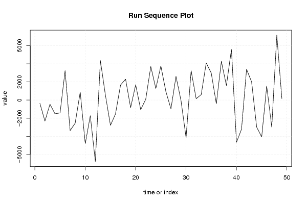
| Title produced by software | Univariate Explorative Data Analysis | ||||||||||||||||||||||||||||||||||||||||||||||||||||
| Date of computation | Mon, 13 Dec 2010 15:34:16 +0000 | ||||||||||||||||||||||||||||||||||||||||||||||||||||
| Cite this page as follows | Statistical Computations at FreeStatistics.org, Office for Research Development and Education, URL https://freestatistics.org/blog/index.php?v=date/2010/Dec/13/t1292254466o6zl9w2nczdynf7.htm/, Retrieved Mon, 06 May 2024 12:54:22 +0000 | ||||||||||||||||||||||||||||||||||||||||||||||||||||
| Statistical Computations at FreeStatistics.org, Office for Research Development and Education, URL https://freestatistics.org/blog/index.php?pk=108960, Retrieved Mon, 06 May 2024 12:54:22 +0000 | |||||||||||||||||||||||||||||||||||||||||||||||||||||
| QR Codes: | |||||||||||||||||||||||||||||||||||||||||||||||||||||
|
| |||||||||||||||||||||||||||||||||||||||||||||||||||||
| Original text written by user: | |||||||||||||||||||||||||||||||||||||||||||||||||||||
| IsPrivate? | No (this computation is public) | ||||||||||||||||||||||||||||||||||||||||||||||||||||
| User-defined keywords | |||||||||||||||||||||||||||||||||||||||||||||||||||||
| Estimated Impact | 151 | ||||||||||||||||||||||||||||||||||||||||||||||||||||
Tree of Dependent Computations | |||||||||||||||||||||||||||||||||||||||||||||||||||||
| Family? (F = Feedback message, R = changed R code, M = changed R Module, P = changed Parameters, D = changed Data) | |||||||||||||||||||||||||||||||||||||||||||||||||||||
| - [Univariate Data Series] [data set] [2008-12-01 19:54:57] [b98453cac15ba1066b407e146608df68] - RMP [Spectral Analysis] [Unemployment] [2010-11-29 09:27:34] [b98453cac15ba1066b407e146608df68] - PD [Spectral Analysis] [Workshop 9 CP (1)] [2010-12-07 15:31:19] [a9e130f95bad0a0597234e75c6380c5a] - [Spectral Analysis] [] [2010-12-07 22:07:26] [afdb2fc47981b6a655b732edc8065db9] - RMPD [Standard Deviation-Mean Plot] [] [2010-12-12 13:55:03] [afdb2fc47981b6a655b732edc8065db9] - RMPD [Univariate Explorative Data Analysis] [] [2010-12-13 15:34:16] [297722d8c88c4886be8e106c47d8f3cc] [Current] | |||||||||||||||||||||||||||||||||||||||||||||||||||||
| Feedback Forum | |||||||||||||||||||||||||||||||||||||||||||||||||||||
Post a new message | |||||||||||||||||||||||||||||||||||||||||||||||||||||
Dataset | |||||||||||||||||||||||||||||||||||||||||||||||||||||
| Dataseries X: | |||||||||||||||||||||||||||||||||||||||||||||||||||||
-359.571607953986 -2313.40174157408 -458.909041234261 -1511.62520054540 -1412.05101907477 3230.73156376355 -3359.59417563836 -2541.21894821932 872.44414461875 -4810.24424730606 -1719.68834437048 -6765.69231129807 4349.73058653668 540.896815335916 -2779.55375248146 -1525.85298806976 1655.44443186453 2302.85011810251 -837.776439784218 1692.87048596592 -1059.92175870099 91.2248118790486 3701.24902827296 1277.781090107 3758.70389605239 927.892916117894 -968.46413469261 2612.52020748951 -67.9700052554981 -4137.99067058662 3239.07295330528 151.781042841903 597.433769339769 4088.59661045384 2965.97886009382 -404.462070874797 4261.25490001266 1607.61904941779 5571.51047223473 -4651.92096188192 -3206.29864576434 3397.26719770752 2004.89246118837 -2974.16877824417 -4061.09181487588 1539.20943989673 -2972.96243506618 7150.15243163015 167.131979535770 | |||||||||||||||||||||||||||||||||||||||||||||||||||||
Tables (Output of Computation) | |||||||||||||||||||||||||||||||||||||||||||||||||||||
| |||||||||||||||||||||||||||||||||||||||||||||||||||||
Figures (Output of Computation) | |||||||||||||||||||||||||||||||||||||||||||||||||||||
Input Parameters & R Code | |||||||||||||||||||||||||||||||||||||||||||||||||||||
| Parameters (Session): | |||||||||||||||||||||||||||||||||||||||||||||||||||||
| par1 = FALSE ; par2 = 1 ; par3 = 1 ; par4 = 1 ; par5 = 12 ; par6 = 3 ; par7 = 1 ; par8 = 2 ; par9 = 1 ; | |||||||||||||||||||||||||||||||||||||||||||||||||||||
| Parameters (R input): | |||||||||||||||||||||||||||||||||||||||||||||||||||||
| par1 = 0 ; par2 = 36 ; | |||||||||||||||||||||||||||||||||||||||||||||||||||||
| R code (references can be found in the software module): | |||||||||||||||||||||||||||||||||||||||||||||||||||||
par1 <- as.numeric(par1) | |||||||||||||||||||||||||||||||||||||||||||||||||||||