Repository of Reproducible Computations

Free Statistics

of Irreproducible Research!

Author's title

Author

*The author of this computation has been verified*

R Software Module

rwasp_autocorrelation.wasp

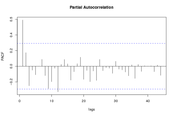
Title produced by software

(Partial) Autocorrelation Function

Date of computation

Mon, 13 Dec 2010 10:05:17 +0000

Cite this page as follows

Statistical Computations at FreeStatistics.org, Office for Research Development and Education, URL https://freestatistics.org/blog/index.php?v=date/2010/Dec/13/t1292234624ng9mvukh4g48gw6.htm/, Retrieved Mon, 06 May 2024 10:52:37 +0000

Statistical Computations at FreeStatistics.org, Office for Research Development and Education, URL https://freestatistics.org/blog/index.php?pk=108750, Retrieved Mon, 06 May 2024 10:52:37 +0000

QR Codes:

Paste this QR Code to cite your computation.

Original text written by user:

IsPrivate?

No (this computation is public)

User-defined keywords

Estimated Impact

163

Family? (F = Feedback message, R = changed R code, M = changed R Module, P = changed Parameters, D = changed Data)

-     [(Partial) Autocorrelation Function] [] [2010-12-13 08:35:23] [21eff0c210342db4afbdafe426a7c254]
-   PD  [(Partial) Autocorrelation Function] [] [2010-12-13 09:29:04] [21eff0c210342db4afbdafe426a7c254]
-    D      [(Partial) Autocorrelation Function] [] [2010-12-13 10:05:17] [81d69fb83507cea26168920232cdff1b] [Current]
- RM D        [Variance Reduction Matrix] [] [2010-12-13 10:10:55] [21eff0c210342db4afbdafe426a7c254] 
- RM D        [Standard Deviation-Mean Plot] [] [2010-12-13 10:21:08] [21eff0c210342db4afbdafe426a7c254] 
- RM D        [Spectral Analysis] [] [2010-12-13 10:28:26] [21eff0c210342db4afbdafe426a7c254] 
- RM D        [Spectral Analysis] [] [2010-12-13 10:28:26] [21eff0c210342db4afbdafe426a7c254] 
-   P           [Spectral Analysis] [] [2010-12-21 18:21:37] [21eff0c210342db4afbdafe426a7c254] 
- RM D        [ARIMA Backward Selection] [] [2010-12-13 10:38:31] [21eff0c210342db4afbdafe426a7c254] 
-   P           [ARIMA Backward Selection] [] [2010-12-13 20:34:12] [21eff0c210342db4afbdafe426a7c254] 
- RM D        [ARIMA Forecasting] [] [2010-12-13 10:48:48] [21eff0c210342db4afbdafe426a7c254] 
-   P           [ARIMA Forecasting] [] [2010-12-13 20:48:40] [21eff0c210342db4afbdafe426a7c254] 
- RMPD          [Univariate Data Series] [] [2010-12-13 20:53:52] [21eff0c210342db4afbdafe426a7c254] 
- RMPD            [Histogram] [] [2010-12-14 14:33:39] [21eff0c210342db4afbdafe426a7c254] 
- RMPD              [Univariate Explorative Data Analysis] [] [2010-12-16 14:06:01] [21eff0c210342db4afbdafe426a7c254] 
- RMPD              [Univariate Data Series] [] [2010-12-16 14:19:11] [de4adef75375d243bafd27c3fb0ddf4c] 
-   PD              [Histogram] [] [2010-12-16 14:23:25] [de4adef75375d243bafd27c3fb0ddf4c] 
- RMPD              [Univariate Explorative Data Analysis] [] [2010-12-16 14:27:05] [de4adef75375d243bafd27c3fb0ddf4c] 
-    D                [Univariate Explorative Data Analysis] [] [2010-12-20 18:48:19] [de4adef75375d243bafd27c3fb0ddf4c] 
- RMPD                [(Partial) Autocorrelation Function] [] [2010-12-20 19:31:04] [de4adef75375d243bafd27c3fb0ddf4c] 
- RMPD                [(Partial) Autocorrelation Function] [] [2010-12-20 19:46:13] [de4adef75375d243bafd27c3fb0ddf4c] 
-   P                   [(Partial) Autocorrelation Function] [] [2010-12-21 15:20:18] [de4adef75375d243bafd27c3fb0ddf4c] 
- RMPD                [Variance Reduction Matrix] [] [2010-12-20 20:00:09] [de4adef75375d243bafd27c3fb0ddf4c] 
- RMPD                [Standard Deviation-Mean Plot] [] [2010-12-20 20:07:24] [de4adef75375d243bafd27c3fb0ddf4c] 
- RMPD                [Spectral Analysis] [] [2010-12-20 20:14:04] [de4adef75375d243bafd27c3fb0ddf4c] 
-   P                   [Spectral Analysis] [] [2010-12-21 16:58:39] [de4adef75375d243bafd27c3fb0ddf4c] 
- RMPD                [Univariate Data Series] [] [2010-12-20 20:24:23] [de4adef75375d243bafd27c3fb0ddf4c] 
-   PD                [Univariate Explorative Data Analysis] [] [2010-12-20 20:29:24] [de4adef75375d243bafd27c3fb0ddf4c] 
-   P                   [Univariate Explorative Data Analysis] [] [2010-12-21 15:07:46] [de4adef75375d243bafd27c3fb0ddf4c] 
- RMPD                [ARIMA Backward Selection] [] [2010-12-20 20:35:32] [de4adef75375d243bafd27c3fb0ddf4c] 
- RMPD                [ARIMA Forecasting] [] [2010-12-20 20:44:58] [de4adef75375d243bafd27c3fb0ddf4c] 
- RMPD              [Variance Reduction Matrix] [] [2010-12-16 14:36:01] [de4adef75375d243bafd27c3fb0ddf4c] 
- RMPD          [Univariate Data Series] [] [2010-12-13 21:02:07] [21eff0c210342db4afbdafe426a7c254] 
-   PD            [Univariate Data Series] [] [2010-12-20 19:00:31] [de4adef75375d243bafd27c3fb0ddf4c] 
- RMPD            [Variance Reduction Matrix] [] [2010-12-20 19:12:17] [de4adef75375d243bafd27c3fb0ddf4c] 
- RMPD          [Central Tendency] [] [2010-12-13 21:04:38] [21eff0c210342db4afbdafe426a7c254] 
- RMPD          [Central Tendency] [] [2010-12-13 21:08:56] [21eff0c210342db4afbdafe426a7c254] 

Feedback Forum

Post a new message

Dataseries X:

Download CSV

Histogram

Boxplots

Summary of computational transaction
Raw Input	view raw input (R code)
Raw Output	view raw output of R engine
Computing time	2 seconds
R Server	'Gwilym Jenkins' @ 72.249.127.135

\begin{tabular}{lllllllll}
\hline
Summary of computational transaction \tabularnewline
Raw Input & view raw input (R code)  \tabularnewline
Raw Output & view raw output of R engine  \tabularnewline
Computing time & 2 seconds \tabularnewline
R Server & 'Gwilym Jenkins' @ 72.249.127.135 \tabularnewline
\hline
\end{tabular}
%Source: https://freestatistics.org/blog/index.php?pk=108750&T=0

[TABLE]
[ROW][C]Summary of computational transaction[/C][/ROW]
[ROW][C]Raw Input[/C][C]view raw input (R code) [/C][/ROW]
[ROW][C]Raw Output[/C][C]view raw output of R engine [/C][/ROW]
[ROW][C]Computing time[/C][C]2 seconds[/C][/ROW]
[ROW][C]R Server[/C][C]'Gwilym Jenkins' @ 72.249.127.135[/C][/ROW]
[/TABLE]
Source: https://freestatistics.org/blog/index.php?pk=108750&T=0

Globally Unique Identifier (entire table): ba.freestatistics.org/blog/index.php?pk=108750&T=0

As an alternative you can also use a QR Code:

The GUIDs for individual cells are displayed in the table below:

Summary of computational transaction
Raw Input	view raw input (R code)
Raw Output	view raw output of R engine
Computing time	2 seconds
R Server	'Gwilym Jenkins' @ 72.249.127.135

Autocorrelation Function
Time lag k	ACF(k)	T-STAT	P-value
1	0.590488	3.9611	0.000132
2	0.461694	3.0971	0.00168
3	0.169735	1.1386	0.130444
4	0.048773	0.3272	0.372524
5	-0.119687	-0.8029	0.213131
6	-0.141588	-0.9498	0.173643
7	-0.114438	-0.7677	0.223345
8	-0.138301	-0.9278	0.179243
9	-0.253713	-1.702	0.047832
10	-0.348417	-2.3373	0.011967
11	-0.367962	-2.4684	0.008719
12	-0.512594	-3.4386	0.000635
13	-0.393908	-2.6424	0.005642
14	-0.27128	-1.8198	0.037722
15	-0.041993	-0.2817	0.389733
16	-0.016878	-0.1132	0.455179
17	0.084277	0.5654	0.287322
18	0.129132	0.8662	0.195475
19	0.199808	1.3404	0.09343
20	0.101708	0.6823	0.24928
21	0.174174	1.1684	0.1244
22	0.120785	0.8102	0.211031
23	0.131423	0.8816	0.191337
24	0.034149	0.2291	0.409923
25	0.098351	0.6598	0.256385
26	0.052055	0.3492	0.364286
27	0.017594	0.118	0.453287
28	0.002789	0.0187	0.492578
29	-0.006354	-0.0426	0.483096
30	0.025857	0.1735	0.431537
31	-0.085902	-0.5762	0.28366
32	-0.034059	-0.2285	0.410156
33	-0.067165	-0.4506	0.327237
34	-0.024722	-0.1658	0.434513
35	-0.04155	-0.2787	0.390867
36	0.006734	0.0452	0.482084
37	0.007724	0.0518	0.479453
38	0.000668	0.0045	0.498223
39	-0.022252	-0.1493	0.441003
40	0.024474	0.1642	0.435165
41	0.025702	0.1724	0.431942
42	-0.013291	-0.0892	0.464677
43	0.014852	0.0996	0.460541
44	-0.006893	-0.0462	0.481662
45	NA	NA	NA
46	NA	NA	NA
47	NA	NA	NA
48	NA	NA	NA

\begin{tabular}{lllllllll}
\hline
Autocorrelation Function \tabularnewline
Time lag k & ACF(k) & T-STAT & P-value \tabularnewline
1 & 0.590488 & 3.9611 & 0.000132 \tabularnewline
2 & 0.461694 & 3.0971 & 0.00168 \tabularnewline
3 & 0.169735 & 1.1386 & 0.130444 \tabularnewline
4 & 0.048773 & 0.3272 & 0.372524 \tabularnewline
5 & -0.119687 & -0.8029 & 0.213131 \tabularnewline
6 & -0.141588 & -0.9498 & 0.173643 \tabularnewline
7 & -0.114438 & -0.7677 & 0.223345 \tabularnewline
8 & -0.138301 & -0.9278 & 0.179243 \tabularnewline
9 & -0.253713 & -1.702 & 0.047832 \tabularnewline
10 & -0.348417 & -2.3373 & 0.011967 \tabularnewline
11 & -0.367962 & -2.4684 & 0.008719 \tabularnewline
12 & -0.512594 & -3.4386 & 0.000635 \tabularnewline
13 & -0.393908 & -2.6424 & 0.005642 \tabularnewline
14 & -0.27128 & -1.8198 & 0.037722 \tabularnewline
15 & -0.041993 & -0.2817 & 0.389733 \tabularnewline
16 & -0.016878 & -0.1132 & 0.455179 \tabularnewline
17 & 0.084277 & 0.5654 & 0.287322 \tabularnewline
18 & 0.129132 & 0.8662 & 0.195475 \tabularnewline
19 & 0.199808 & 1.3404 & 0.09343 \tabularnewline
20 & 0.101708 & 0.6823 & 0.24928 \tabularnewline
21 & 0.174174 & 1.1684 & 0.1244 \tabularnewline
22 & 0.120785 & 0.8102 & 0.211031 \tabularnewline
23 & 0.131423 & 0.8816 & 0.191337 \tabularnewline
24 & 0.034149 & 0.2291 & 0.409923 \tabularnewline
25 & 0.098351 & 0.6598 & 0.256385 \tabularnewline
26 & 0.052055 & 0.3492 & 0.364286 \tabularnewline
27 & 0.017594 & 0.118 & 0.453287 \tabularnewline
28 & 0.002789 & 0.0187 & 0.492578 \tabularnewline
29 & -0.006354 & -0.0426 & 0.483096 \tabularnewline
30 & 0.025857 & 0.1735 & 0.431537 \tabularnewline
31 & -0.085902 & -0.5762 & 0.28366 \tabularnewline
32 & -0.034059 & -0.2285 & 0.410156 \tabularnewline
33 & -0.067165 & -0.4506 & 0.327237 \tabularnewline
34 & -0.024722 & -0.1658 & 0.434513 \tabularnewline
35 & -0.04155 & -0.2787 & 0.390867 \tabularnewline
36 & 0.006734 & 0.0452 & 0.482084 \tabularnewline
37 & 0.007724 & 0.0518 & 0.479453 \tabularnewline
38 & 0.000668 & 0.0045 & 0.498223 \tabularnewline
39 & -0.022252 & -0.1493 & 0.441003 \tabularnewline
40 & 0.024474 & 0.1642 & 0.435165 \tabularnewline
41 & 0.025702 & 0.1724 & 0.431942 \tabularnewline
42 & -0.013291 & -0.0892 & 0.464677 \tabularnewline
43 & 0.014852 & 0.0996 & 0.460541 \tabularnewline
44 & -0.006893 & -0.0462 & 0.481662 \tabularnewline
45 & NA & NA & NA \tabularnewline
46 & NA & NA & NA \tabularnewline
47 & NA & NA & NA \tabularnewline
48 & NA & NA & NA \tabularnewline
\hline
\end{tabular}
%Source: https://freestatistics.org/blog/index.php?pk=108750&T=1

[TABLE]
[ROW][C]Autocorrelation Function[/C][/ROW]
[ROW][C]Time lag k[/C][C]ACF(k)[/C][C]T-STAT[/C][C]P-value[/C][/ROW]
[ROW][C]1[/C][C]0.590488[/C][C]3.9611[/C][C]0.000132[/C][/ROW]
[ROW][C]2[/C][C]0.461694[/C][C]3.0971[/C][C]0.00168[/C][/ROW]
[ROW][C]3[/C][C]0.169735[/C][C]1.1386[/C][C]0.130444[/C][/ROW]
[ROW][C]4[/C][C]0.048773[/C][C]0.3272[/C][C]0.372524[/C][/ROW]
[ROW][C]5[/C][C]-0.119687[/C][C]-0.8029[/C][C]0.213131[/C][/ROW]
[ROW][C]6[/C][C]-0.141588[/C][C]-0.9498[/C][C]0.173643[/C][/ROW]
[ROW][C]7[/C][C]-0.114438[/C][C]-0.7677[/C][C]0.223345[/C][/ROW]
[ROW][C]8[/C][C]-0.138301[/C][C]-0.9278[/C][C]0.179243[/C][/ROW]
[ROW][C]9[/C][C]-0.253713[/C][C]-1.702[/C][C]0.047832[/C][/ROW]
[ROW][C]10[/C][C]-0.348417[/C][C]-2.3373[/C][C]0.011967[/C][/ROW]
[ROW][C]11[/C][C]-0.367962[/C][C]-2.4684[/C][C]0.008719[/C][/ROW]
[ROW][C]12[/C][C]-0.512594[/C][C]-3.4386[/C][C]0.000635[/C][/ROW]
[ROW][C]13[/C][C]-0.393908[/C][C]-2.6424[/C][C]0.005642[/C][/ROW]
[ROW][C]14[/C][C]-0.27128[/C][C]-1.8198[/C][C]0.037722[/C][/ROW]
[ROW][C]15[/C][C]-0.041993[/C][C]-0.2817[/C][C]0.389733[/C][/ROW]
[ROW][C]16[/C][C]-0.016878[/C][C]-0.1132[/C][C]0.455179[/C][/ROW]
[ROW][C]17[/C][C]0.084277[/C][C]0.5654[/C][C]0.287322[/C][/ROW]
[ROW][C]18[/C][C]0.129132[/C][C]0.8662[/C][C]0.195475[/C][/ROW]
[ROW][C]19[/C][C]0.199808[/C][C]1.3404[/C][C]0.09343[/C][/ROW]
[ROW][C]20[/C][C]0.101708[/C][C]0.6823[/C][C]0.24928[/C][/ROW]
[ROW][C]21[/C][C]0.174174[/C][C]1.1684[/C][C]0.1244[/C][/ROW]
[ROW][C]22[/C][C]0.120785[/C][C]0.8102[/C][C]0.211031[/C][/ROW]
[ROW][C]23[/C][C]0.131423[/C][C]0.8816[/C][C]0.191337[/C][/ROW]
[ROW][C]24[/C][C]0.034149[/C][C]0.2291[/C][C]0.409923[/C][/ROW]
[ROW][C]25[/C][C]0.098351[/C][C]0.6598[/C][C]0.256385[/C][/ROW]
[ROW][C]26[/C][C]0.052055[/C][C]0.3492[/C][C]0.364286[/C][/ROW]
[ROW][C]27[/C][C]0.017594[/C][C]0.118[/C][C]0.453287[/C][/ROW]
[ROW][C]28[/C][C]0.002789[/C][C]0.0187[/C][C]0.492578[/C][/ROW]
[ROW][C]29[/C][C]-0.006354[/C][C]-0.0426[/C][C]0.483096[/C][/ROW]
[ROW][C]30[/C][C]0.025857[/C][C]0.1735[/C][C]0.431537[/C][/ROW]
[ROW][C]31[/C][C]-0.085902[/C][C]-0.5762[/C][C]0.28366[/C][/ROW]
[ROW][C]32[/C][C]-0.034059[/C][C]-0.2285[/C][C]0.410156[/C][/ROW]
[ROW][C]33[/C][C]-0.067165[/C][C]-0.4506[/C][C]0.327237[/C][/ROW]
[ROW][C]34[/C][C]-0.024722[/C][C]-0.1658[/C][C]0.434513[/C][/ROW]
[ROW][C]35[/C][C]-0.04155[/C][C]-0.2787[/C][C]0.390867[/C][/ROW]
[ROW][C]36[/C][C]0.006734[/C][C]0.0452[/C][C]0.482084[/C][/ROW]
[ROW][C]37[/C][C]0.007724[/C][C]0.0518[/C][C]0.479453[/C][/ROW]
[ROW][C]38[/C][C]0.000668[/C][C]0.0045[/C][C]0.498223[/C][/ROW]
[ROW][C]39[/C][C]-0.022252[/C][C]-0.1493[/C][C]0.441003[/C][/ROW]
[ROW][C]40[/C][C]0.024474[/C][C]0.1642[/C][C]0.435165[/C][/ROW]
[ROW][C]41[/C][C]0.025702[/C][C]0.1724[/C][C]0.431942[/C][/ROW]
[ROW][C]42[/C][C]-0.013291[/C][C]-0.0892[/C][C]0.464677[/C][/ROW]
[ROW][C]43[/C][C]0.014852[/C][C]0.0996[/C][C]0.460541[/C][/ROW]
[ROW][C]44[/C][C]-0.006893[/C][C]-0.0462[/C][C]0.481662[/C][/ROW]
[ROW][C]45[/C][C]NA[/C][C]NA[/C][C]NA[/C][/ROW]
[ROW][C]46[/C][C]NA[/C][C]NA[/C][C]NA[/C][/ROW]
[ROW][C]47[/C][C]NA[/C][C]NA[/C][C]NA[/C][/ROW]
[ROW][C]48[/C][C]NA[/C][C]NA[/C][C]NA[/C][/ROW]
[/TABLE]
Source: https://freestatistics.org/blog/index.php?pk=108750&T=1

Globally Unique Identifier (entire table): ba.freestatistics.org/blog/index.php?pk=108750&T=1

As an alternative you can also use a QR Code:

The GUIDs for individual cells are displayed in the table below:

Autocorrelation Function
Time lag k	ACF(k)	T-STAT	P-value
1	0.590488	3.9611	0.000132
2	0.461694	3.0971	0.00168
3	0.169735	1.1386	0.130444
4	0.048773	0.3272	0.372524
5	-0.119687	-0.8029	0.213131
6	-0.141588	-0.9498	0.173643
7	-0.114438	-0.7677	0.223345
8	-0.138301	-0.9278	0.179243
9	-0.253713	-1.702	0.047832
10	-0.348417	-2.3373	0.011967
11	-0.367962	-2.4684	0.008719
12	-0.512594	-3.4386	0.000635
13	-0.393908	-2.6424	0.005642
14	-0.27128	-1.8198	0.037722
15	-0.041993	-0.2817	0.389733
16	-0.016878	-0.1132	0.455179
17	0.084277	0.5654	0.287322
18	0.129132	0.8662	0.195475
19	0.199808	1.3404	0.09343
20	0.101708	0.6823	0.24928
21	0.174174	1.1684	0.1244
22	0.120785	0.8102	0.211031
23	0.131423	0.8816	0.191337
24	0.034149	0.2291	0.409923
25	0.098351	0.6598	0.256385
26	0.052055	0.3492	0.364286
27	0.017594	0.118	0.453287
28	0.002789	0.0187	0.492578
29	-0.006354	-0.0426	0.483096
30	0.025857	0.1735	0.431537
31	-0.085902	-0.5762	0.28366
32	-0.034059	-0.2285	0.410156
33	-0.067165	-0.4506	0.327237
34	-0.024722	-0.1658	0.434513
35	-0.04155	-0.2787	0.390867
36	0.006734	0.0452	0.482084
37	0.007724	0.0518	0.479453
38	0.000668	0.0045	0.498223
39	-0.022252	-0.1493	0.441003
40	0.024474	0.1642	0.435165
41	0.025702	0.1724	0.431942
42	-0.013291	-0.0892	0.464677
43	0.014852	0.0996	0.460541
44	-0.006893	-0.0462	0.481662
45	NA	NA	NA
46	NA	NA	NA
47	NA	NA	NA
48	NA	NA	NA

Partial Autocorrelation Function
Time lag k	PACF(k)	T-STAT	P-value
1	0.590488	3.9611	0.000132
2	0.173521	1.164	0.125277
3	-0.250186	-1.6783	0.050111
4	-0.050971	-0.3419	0.366999
5	-0.109405	-0.7339	0.233406
6	-0.000179	-0.0012	0.499523
7	0.087881	0.5895	0.279229
8	-0.120281	-0.8069	0.211993
9	-0.285472	-1.915	0.030931
10	-0.198162	-1.3293	0.095222
11	-0.025898	-0.1737	0.431428
12	-0.327124	-2.1944	0.016704
13	0.023613	0.1584	0.437424
14	0.086728	0.5818	0.281806
15	0.030538	0.2049	0.419304
16	-0.17825	-1.1957	0.11903
17	-0.070624	-0.4738	0.318982
18	0.032465	0.2178	0.414293
19	0.115402	0.7741	0.221447
20	-0.168535	-1.1306	0.132114
21	-0.054559	-0.366	0.358043
22	-0.198232	-1.3298	0.095147
23	-0.061233	-0.4108	0.341598
24	-0.181789	-1.2195	0.114508
25	0.08719	0.5849	0.280772
26	-0.057557	-0.3861	0.350619
27	-0.018283	-0.1226	0.451466
28	-0.025627	-0.1719	0.432139
29	-0.091416	-0.6132	0.271403
30	0.063249	0.4243	0.336689
31	-0.038063	-0.2553	0.399815
32	-0.047594	-0.3193	0.3755
33	-0.0742	-0.4977	0.310542
34	-0.122539	-0.822	0.207702
35	0.018342	0.123	0.451312
36	-0.156486	-1.0497	0.149722
37	0.023093	0.1549	0.438791
38	-0.067022	-0.4496	0.327579
39	0.00622	0.0417	0.483452
40	0.000928	0.0062	0.49753
41	0.005018	0.0337	0.486649
42	-0.070135	-0.4705	0.320143
43	0.014726	0.0988	0.460874
44	-0.11764	-0.7891	0.217081
45	NA	NA	NA
46	NA	NA	NA
47	NA	NA	NA
48	NA	NA	NA

\begin{tabular}{lllllllll}
\hline
Partial Autocorrelation Function \tabularnewline
Time lag k & PACF(k) & T-STAT & P-value \tabularnewline
1 & 0.590488 & 3.9611 & 0.000132 \tabularnewline
2 & 0.173521 & 1.164 & 0.125277 \tabularnewline
3 & -0.250186 & -1.6783 & 0.050111 \tabularnewline
4 & -0.050971 & -0.3419 & 0.366999 \tabularnewline
5 & -0.109405 & -0.7339 & 0.233406 \tabularnewline
6 & -0.000179 & -0.0012 & 0.499523 \tabularnewline
7 & 0.087881 & 0.5895 & 0.279229 \tabularnewline
8 & -0.120281 & -0.8069 & 0.211993 \tabularnewline
9 & -0.285472 & -1.915 & 0.030931 \tabularnewline
10 & -0.198162 & -1.3293 & 0.095222 \tabularnewline
11 & -0.025898 & -0.1737 & 0.431428 \tabularnewline
12 & -0.327124 & -2.1944 & 0.016704 \tabularnewline
13 & 0.023613 & 0.1584 & 0.437424 \tabularnewline
14 & 0.086728 & 0.5818 & 0.281806 \tabularnewline
15 & 0.030538 & 0.2049 & 0.419304 \tabularnewline
16 & -0.17825 & -1.1957 & 0.11903 \tabularnewline
17 & -0.070624 & -0.4738 & 0.318982 \tabularnewline
18 & 0.032465 & 0.2178 & 0.414293 \tabularnewline
19 & 0.115402 & 0.7741 & 0.221447 \tabularnewline
20 & -0.168535 & -1.1306 & 0.132114 \tabularnewline
21 & -0.054559 & -0.366 & 0.358043 \tabularnewline
22 & -0.198232 & -1.3298 & 0.095147 \tabularnewline
23 & -0.061233 & -0.4108 & 0.341598 \tabularnewline
24 & -0.181789 & -1.2195 & 0.114508 \tabularnewline
25 & 0.08719 & 0.5849 & 0.280772 \tabularnewline
26 & -0.057557 & -0.3861 & 0.350619 \tabularnewline
27 & -0.018283 & -0.1226 & 0.451466 \tabularnewline
28 & -0.025627 & -0.1719 & 0.432139 \tabularnewline
29 & -0.091416 & -0.6132 & 0.271403 \tabularnewline
30 & 0.063249 & 0.4243 & 0.336689 \tabularnewline
31 & -0.038063 & -0.2553 & 0.399815 \tabularnewline
32 & -0.047594 & -0.3193 & 0.3755 \tabularnewline
33 & -0.0742 & -0.4977 & 0.310542 \tabularnewline
34 & -0.122539 & -0.822 & 0.207702 \tabularnewline
35 & 0.018342 & 0.123 & 0.451312 \tabularnewline
36 & -0.156486 & -1.0497 & 0.149722 \tabularnewline
37 & 0.023093 & 0.1549 & 0.438791 \tabularnewline
38 & -0.067022 & -0.4496 & 0.327579 \tabularnewline
39 & 0.00622 & 0.0417 & 0.483452 \tabularnewline
40 & 0.000928 & 0.0062 & 0.49753 \tabularnewline
41 & 0.005018 & 0.0337 & 0.486649 \tabularnewline
42 & -0.070135 & -0.4705 & 0.320143 \tabularnewline
43 & 0.014726 & 0.0988 & 0.460874 \tabularnewline
44 & -0.11764 & -0.7891 & 0.217081 \tabularnewline
45 & NA & NA & NA \tabularnewline
46 & NA & NA & NA \tabularnewline
47 & NA & NA & NA \tabularnewline
48 & NA & NA & NA \tabularnewline
\hline
\end{tabular}
%Source: https://freestatistics.org/blog/index.php?pk=108750&T=2

[TABLE]
[ROW][C]Partial Autocorrelation Function[/C][/ROW]
[ROW][C]Time lag k[/C][C]PACF(k)[/C][C]T-STAT[/C][C]P-value[/C][/ROW]
[ROW][C]1[/C][C]0.590488[/C][C]3.9611[/C][C]0.000132[/C][/ROW]
[ROW][C]2[/C][C]0.173521[/C][C]1.164[/C][C]0.125277[/C][/ROW]
[ROW][C]3[/C][C]-0.250186[/C][C]-1.6783[/C][C]0.050111[/C][/ROW]
[ROW][C]4[/C][C]-0.050971[/C][C]-0.3419[/C][C]0.366999[/C][/ROW]
[ROW][C]5[/C][C]-0.109405[/C][C]-0.7339[/C][C]0.233406[/C][/ROW]
[ROW][C]6[/C][C]-0.000179[/C][C]-0.0012[/C][C]0.499523[/C][/ROW]
[ROW][C]7[/C][C]0.087881[/C][C]0.5895[/C][C]0.279229[/C][/ROW]
[ROW][C]8[/C][C]-0.120281[/C][C]-0.8069[/C][C]0.211993[/C][/ROW]
[ROW][C]9[/C][C]-0.285472[/C][C]-1.915[/C][C]0.030931[/C][/ROW]
[ROW][C]10[/C][C]-0.198162[/C][C]-1.3293[/C][C]0.095222[/C][/ROW]
[ROW][C]11[/C][C]-0.025898[/C][C]-0.1737[/C][C]0.431428[/C][/ROW]
[ROW][C]12[/C][C]-0.327124[/C][C]-2.1944[/C][C]0.016704[/C][/ROW]
[ROW][C]13[/C][C]0.023613[/C][C]0.1584[/C][C]0.437424[/C][/ROW]
[ROW][C]14[/C][C]0.086728[/C][C]0.5818[/C][C]0.281806[/C][/ROW]
[ROW][C]15[/C][C]0.030538[/C][C]0.2049[/C][C]0.419304[/C][/ROW]
[ROW][C]16[/C][C]-0.17825[/C][C]-1.1957[/C][C]0.11903[/C][/ROW]
[ROW][C]17[/C][C]-0.070624[/C][C]-0.4738[/C][C]0.318982[/C][/ROW]
[ROW][C]18[/C][C]0.032465[/C][C]0.2178[/C][C]0.414293[/C][/ROW]
[ROW][C]19[/C][C]0.115402[/C][C]0.7741[/C][C]0.221447[/C][/ROW]
[ROW][C]20[/C][C]-0.168535[/C][C]-1.1306[/C][C]0.132114[/C][/ROW]
[ROW][C]21[/C][C]-0.054559[/C][C]-0.366[/C][C]0.358043[/C][/ROW]
[ROW][C]22[/C][C]-0.198232[/C][C]-1.3298[/C][C]0.095147[/C][/ROW]
[ROW][C]23[/C][C]-0.061233[/C][C]-0.4108[/C][C]0.341598[/C][/ROW]
[ROW][C]24[/C][C]-0.181789[/C][C]-1.2195[/C][C]0.114508[/C][/ROW]
[ROW][C]25[/C][C]0.08719[/C][C]0.5849[/C][C]0.280772[/C][/ROW]
[ROW][C]26[/C][C]-0.057557[/C][C]-0.3861[/C][C]0.350619[/C][/ROW]
[ROW][C]27[/C][C]-0.018283[/C][C]-0.1226[/C][C]0.451466[/C][/ROW]
[ROW][C]28[/C][C]-0.025627[/C][C]-0.1719[/C][C]0.432139[/C][/ROW]
[ROW][C]29[/C][C]-0.091416[/C][C]-0.6132[/C][C]0.271403[/C][/ROW]
[ROW][C]30[/C][C]0.063249[/C][C]0.4243[/C][C]0.336689[/C][/ROW]
[ROW][C]31[/C][C]-0.038063[/C][C]-0.2553[/C][C]0.399815[/C][/ROW]
[ROW][C]32[/C][C]-0.047594[/C][C]-0.3193[/C][C]0.3755[/C][/ROW]
[ROW][C]33[/C][C]-0.0742[/C][C]-0.4977[/C][C]0.310542[/C][/ROW]
[ROW][C]34[/C][C]-0.122539[/C][C]-0.822[/C][C]0.207702[/C][/ROW]
[ROW][C]35[/C][C]0.018342[/C][C]0.123[/C][C]0.451312[/C][/ROW]
[ROW][C]36[/C][C]-0.156486[/C][C]-1.0497[/C][C]0.149722[/C][/ROW]
[ROW][C]37[/C][C]0.023093[/C][C]0.1549[/C][C]0.438791[/C][/ROW]
[ROW][C]38[/C][C]-0.067022[/C][C]-0.4496[/C][C]0.327579[/C][/ROW]
[ROW][C]39[/C][C]0.00622[/C][C]0.0417[/C][C]0.483452[/C][/ROW]
[ROW][C]40[/C][C]0.000928[/C][C]0.0062[/C][C]0.49753[/C][/ROW]
[ROW][C]41[/C][C]0.005018[/C][C]0.0337[/C][C]0.486649[/C][/ROW]
[ROW][C]42[/C][C]-0.070135[/C][C]-0.4705[/C][C]0.320143[/C][/ROW]
[ROW][C]43[/C][C]0.014726[/C][C]0.0988[/C][C]0.460874[/C][/ROW]
[ROW][C]44[/C][C]-0.11764[/C][C]-0.7891[/C][C]0.217081[/C][/ROW]
[ROW][C]45[/C][C]NA[/C][C]NA[/C][C]NA[/C][/ROW]
[ROW][C]46[/C][C]NA[/C][C]NA[/C][C]NA[/C][/ROW]
[ROW][C]47[/C][C]NA[/C][C]NA[/C][C]NA[/C][/ROW]
[ROW][C]48[/C][C]NA[/C][C]NA[/C][C]NA[/C][/ROW]
[/TABLE]
Source: https://freestatistics.org/blog/index.php?pk=108750&T=2

Globally Unique Identifier (entire table): ba.freestatistics.org/blog/index.php?pk=108750&T=2

As an alternative you can also use a QR Code:

The GUIDs for individual cells are displayed in the table below:

Partial Autocorrelation Function
Time lag k	PACF(k)	T-STAT	P-value
1	0.590488	3.9611	0.000132
2	0.173521	1.164	0.125277
3	-0.250186	-1.6783	0.050111
4	-0.050971	-0.3419	0.366999
5	-0.109405	-0.7339	0.233406
6	-0.000179	-0.0012	0.499523
7	0.087881	0.5895	0.279229
8	-0.120281	-0.8069	0.211993
9	-0.285472	-1.915	0.030931
10	-0.198162	-1.3293	0.095222
11	-0.025898	-0.1737	0.431428
12	-0.327124	-2.1944	0.016704
13	0.023613	0.1584	0.437424
14	0.086728	0.5818	0.281806
15	0.030538	0.2049	0.419304
16	-0.17825	-1.1957	0.11903
17	-0.070624	-0.4738	0.318982
18	0.032465	0.2178	0.414293
19	0.115402	0.7741	0.221447
20	-0.168535	-1.1306	0.132114
21	-0.054559	-0.366	0.358043
22	-0.198232	-1.3298	0.095147
23	-0.061233	-0.4108	0.341598
24	-0.181789	-1.2195	0.114508
25	0.08719	0.5849	0.280772
26	-0.057557	-0.3861	0.350619
27	-0.018283	-0.1226	0.451466
28	-0.025627	-0.1719	0.432139
29	-0.091416	-0.6132	0.271403
30	0.063249	0.4243	0.336689
31	-0.038063	-0.2553	0.399815
32	-0.047594	-0.3193	0.3755
33	-0.0742	-0.4977	0.310542
34	-0.122539	-0.822	0.207702
35	0.018342	0.123	0.451312
36	-0.156486	-1.0497	0.149722
37	0.023093	0.1549	0.438791
38	-0.067022	-0.4496	0.327579
39	0.00622	0.0417	0.483452
40	0.000928	0.0062	0.49753
41	0.005018	0.0337	0.486649
42	-0.070135	-0.4705	0.320143
43	0.014726	0.0988	0.460874
44	-0.11764	-0.7891	0.217081
45	NA	NA	NA
46	NA	NA	NA
47	NA	NA	NA
48	NA	NA	NA

Figure 1

PNG link

Postscript link

PDF link

Figure 2

PNG link

Postscript link

PDF link

Parameters (Session):

par1 = 48 ; par2 = 1 ; par3 = 0 ; par4 = 0 ; par5 = 12 ; par6 = White Noise ; par7 = 0.95 ;

Parameters (R input):

par1 = 48 ; par2 = 1 ; par3 = 1 ; par4 = 1 ; par5 = 12 ; par6 = White Noise ; par7 = 0.95 ;

R code (references can be found in the software module):

if (par1 == 'Default') {
par1 = 10*log10(length(x))
} else {
par1 <- as.numeric(par1)
}
par2 <- as.numeric(par2)
par3 <- as.numeric(par3)
par4 <- as.numeric(par4)
par5 <- as.numeric(par5)
if (par6 == 'White Noise') par6 <- 'white' else par6 <- 'ma'
par7 <- as.numeric(par7)
if (par2 == 0) {
x <- log(x)
} else {
x <- (x ^ par2 - 1) / par2
}
if (par3 > 0) x <- diff(x,lag=1,difference=par3)
if (par4 > 0) x <- diff(x,lag=par5,difference=par4)
bitmap(file='pic1.png')
racf <- acf(x, par1, main='Autocorrelation', xlab='time lag', ylab='ACF', ci.type=par6, ci=par7, sub=paste('(lambda=',par2,', d=',par3,', D=',par4,', CI=', par7, ', CI type=',par6,')',sep=''))
dev.off()
bitmap(file='pic2.png')
rpacf <- pacf(x,par1,main='Partial Autocorrelation',xlab='lags',ylab='PACF')
dev.off()
(myacf <- c(racf$acf))
(mypacf <- c(rpacf$acf))
lengthx <- length(x)
sqrtn <- sqrt(lengthx)
load(file='createtable')
a<-table.start()
a<-table.row.start(a)
a<-table.element(a,'Autocorrelation Function',4,TRUE)
a<-table.row.end(a)
a<-table.row.start(a)
a<-table.element(a,'Time lag k',header=TRUE)
a<-table.element(a,hyperlink('basics.htm','ACF(k)','click here for more information about the Autocorrelation Function'),header=TRUE)
a<-table.element(a,'T-STAT',header=TRUE)
a<-table.element(a,'P-value',header=TRUE)
a<-table.row.end(a)
for (i in 2:(par1+1)) {
a<-table.row.start(a)
a<-table.element(a,i-1,header=TRUE)
a<-table.element(a,round(myacf[i],6))
mytstat <- myacf[i]*sqrtn
a<-table.element(a,round(mytstat,4))
a<-table.element(a,round(1-pt(abs(mytstat),lengthx),6))
a<-table.row.end(a)
}
a<-table.end(a)
table.save(a,file='mytable.tab')
a<-table.start()
a<-table.row.start(a)
a<-table.element(a,'Partial Autocorrelation Function',4,TRUE)
a<-table.row.end(a)
a<-table.row.start(a)
a<-table.element(a,'Time lag k',header=TRUE)
a<-table.element(a,hyperlink('basics.htm','PACF(k)','click here for more information about the Partial Autocorrelation Function'),header=TRUE)
a<-table.element(a,'T-STAT',header=TRUE)
a<-table.element(a,'P-value',header=TRUE)
a<-table.row.end(a)
for (i in 1:par1) {
a<-table.row.start(a)
a<-table.element(a,i,header=TRUE)
a<-table.element(a,round(mypacf[i],6))
mytstat <- mypacf[i]*sqrtn
a<-table.element(a,round(mytstat,4))
a<-table.element(a,round(1-pt(abs(mytstat),lengthx),6))
a<-table.row.end(a)
}
a<-table.end(a)
table.save(a,file='mytable1.tab')

Free Statistics

Description of Statistical Computation

Tree of Dependent Computations

Dataset

Tables (Output of Computation)

Figures (Output of Computation)

Input Parameters & R Code