Repository of Reproducible Computations

Free Statistics

of Irreproducible Research!

Author's title

Author

*The author of this computation has been verified*

R Software Module

rwasp_autocorrelation.wasp

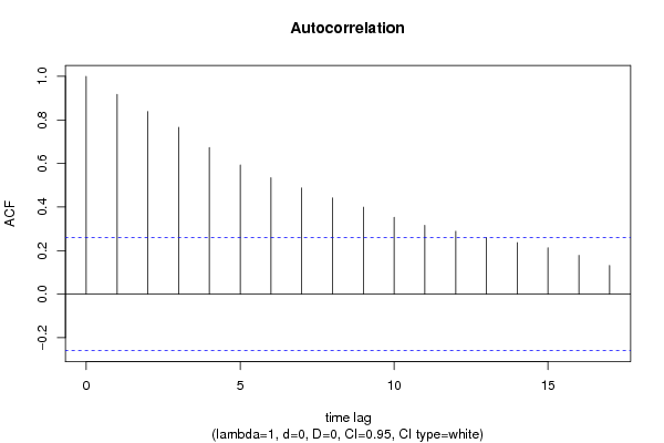
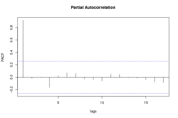
Title produced by software

(Partial) Autocorrelation Function

Date of computation

Mon, 13 Dec 2010 08:35:23 +0000

Cite this page as follows

Statistical Computations at FreeStatistics.org, Office for Research Development and Education, URL https://freestatistics.org/blog/index.php?v=date/2010/Dec/13/t1292229264jvke06wf2kj0qc5.htm/, Retrieved Mon, 06 May 2024 23:29:28 +0000

Statistical Computations at FreeStatistics.org, Office for Research Development and Education, URL https://freestatistics.org/blog/index.php?pk=108698, Retrieved Mon, 06 May 2024 23:29:28 +0000

QR Codes:

Paste this QR Code to cite your computation.

Original text written by user:

IsPrivate?

No (this computation is public)

User-defined keywords

Estimated Impact

173

Family? (F = Feedback message, R = changed R code, M = changed R Module, P = changed Parameters, D = changed Data)

-       [(Partial) Autocorrelation Function] [] [2010-12-13 08:35:23] [81d69fb83507cea26168920232cdff1b] [Current]
-   PD    [(Partial) Autocorrelation Function] [] [2010-12-13 09:14:56] [21eff0c210342db4afbdafe426a7c254] 
-   PD    [(Partial) Autocorrelation Function] [] [2010-12-13 09:17:25] [21eff0c210342db4afbdafe426a7c254] 
-   PD    [(Partial) Autocorrelation Function] [] [2010-12-13 09:19:49] [21eff0c210342db4afbdafe426a7c254] 
-   PD    [(Partial) Autocorrelation Function] [] [2010-12-13 09:24:16] [21eff0c210342db4afbdafe426a7c254] 
-   PD    [(Partial) Autocorrelation Function] [] [2010-12-13 09:29:04] [21eff0c210342db4afbdafe426a7c254] 
-    D      [(Partial) Autocorrelation Function] [] [2010-12-13 09:39:12] [21eff0c210342db4afbdafe426a7c254] 
-   P         [(Partial) Autocorrelation Function] [] [2010-12-13 19:58:53] [21eff0c210342db4afbdafe426a7c254] 
-   PD        [(Partial) Autocorrelation Function] [] [2010-12-13 20:02:45] [21eff0c210342db4afbdafe426a7c254] 
-   PD        [(Partial) Autocorrelation Function] [] [2010-12-13 20:04:16] [21eff0c210342db4afbdafe426a7c254] 
-    D      [(Partial) Autocorrelation Function] [] [2010-12-13 09:51:46] [21eff0c210342db4afbdafe426a7c254] 
-    D      [(Partial) Autocorrelation Function] [] [2010-12-13 09:59:22] [21eff0c210342db4afbdafe426a7c254] 
-    D      [(Partial) Autocorrelation Function] [] [2010-12-13 10:05:17] [21eff0c210342db4afbdafe426a7c254] 
- RM D        [Variance Reduction Matrix] [] [2010-12-13 10:10:55] [21eff0c210342db4afbdafe426a7c254] 
- RM D        [Standard Deviation-Mean Plot] [] [2010-12-13 10:21:08] [21eff0c210342db4afbdafe426a7c254] 
- RM D        [Spectral Analysis] [] [2010-12-13 10:28:26] [21eff0c210342db4afbdafe426a7c254] 
- RM D        [Spectral Analysis] [] [2010-12-13 10:28:26] [21eff0c210342db4afbdafe426a7c254] 
-   P           [Spectral Analysis] [] [2010-12-21 18:21:37] [21eff0c210342db4afbdafe426a7c254] 
- RM D        [ARIMA Backward Selection] [] [2010-12-13 10:38:31] [21eff0c210342db4afbdafe426a7c254] 
-   P           [ARIMA Backward Selection] [] [2010-12-13 20:34:12] [21eff0c210342db4afbdafe426a7c254] 
- RM D        [ARIMA Forecasting] [] [2010-12-13 10:48:48] [21eff0c210342db4afbdafe426a7c254] 
-   P           [ARIMA Forecasting] [] [2010-12-13 20:48:40] [21eff0c210342db4afbdafe426a7c254] 
- RMPD          [Univariate Data Series] [] [2010-12-13 20:53:52] [21eff0c210342db4afbdafe426a7c254] 
- RMPD            [Histogram] [] [2010-12-14 14:33:39] [21eff0c210342db4afbdafe426a7c254] 
- RMPD              [Univariate Explorative Data Analysis] [] [2010-12-16 14:06:01] [21eff0c210342db4afbdafe426a7c254] 
- RMPD              [Univariate Data Series] [] [2010-12-16 14:19:11] [de4adef75375d243bafd27c3fb0ddf4c] 
-   PD              [Histogram] [] [2010-12-16 14:23:25] [de4adef75375d243bafd27c3fb0ddf4c] 
- RMPD              [Univariate Explorative Data Analysis] [] [2010-12-16 14:27:05] [de4adef75375d243bafd27c3fb0ddf4c] 
-    D                [Univariate Explorative Data Analysis] [] [2010-12-20 18:48:19] [de4adef75375d243bafd27c3fb0ddf4c] 
- RMPD                [(Partial) Autocorrelation Function] [] [2010-12-20 19:31:04] [de4adef75375d243bafd27c3fb0ddf4c] 
- RMPD                [(Partial) Autocorrelation Function] [] [2010-12-20 19:46:13] [de4adef75375d243bafd27c3fb0ddf4c] 
-   P                   [(Partial) Autocorrelation Function] [] [2010-12-21 15:20:18] [de4adef75375d243bafd27c3fb0ddf4c] 
- RMPD                [Variance Reduction Matrix] [] [2010-12-20 20:00:09] [de4adef75375d243bafd27c3fb0ddf4c] 
- RMPD                [Standard Deviation-Mean Plot] [] [2010-12-20 20:07:24] [de4adef75375d243bafd27c3fb0ddf4c] 
- RMPD                [Spectral Analysis] [] [2010-12-20 20:14:04] [de4adef75375d243bafd27c3fb0ddf4c] 
-   P                   [Spectral Analysis] [] [2010-12-21 16:58:39] [de4adef75375d243bafd27c3fb0ddf4c] 
- RMPD                [Univariate Data Series] [] [2010-12-20 20:24:23] [de4adef75375d243bafd27c3fb0ddf4c] 
-   PD                [Univariate Explorative Data Analysis] [] [2010-12-20 20:29:24] [de4adef75375d243bafd27c3fb0ddf4c] 
-   P                   [Univariate Explorative Data Analysis] [] [2010-12-21 15:07:46] [de4adef75375d243bafd27c3fb0ddf4c] 
- RMPD                [ARIMA Backward Selection] [] [2010-12-20 20:35:32] [de4adef75375d243bafd27c3fb0ddf4c] 
- RMPD                [ARIMA Forecasting] [] [2010-12-20 20:44:58] [de4adef75375d243bafd27c3fb0ddf4c] 
- RMPD              [Variance Reduction Matrix] [] [2010-12-16 14:36:01] [de4adef75375d243bafd27c3fb0ddf4c] 
- RMPD          [Univariate Data Series] [] [2010-12-13 21:02:07] [21eff0c210342db4afbdafe426a7c254] 
-   PD            [Univariate Data Series] [] [2010-12-20 19:00:31] [de4adef75375d243bafd27c3fb0ddf4c] 
- RMPD            [Variance Reduction Matrix] [] [2010-12-20 19:12:17] [de4adef75375d243bafd27c3fb0ddf4c] 
- RMPD          [Central Tendency] [] [2010-12-13 21:04:38] [21eff0c210342db4afbdafe426a7c254] 
- RMPD          [Central Tendency] [] [2010-12-13 21:08:56] [21eff0c210342db4afbdafe426a7c254] 

Feedback Forum

Post a new message

Dataseries X:

Download CSV

Histogram

Boxplots

Summary of computational transaction
Raw Input	view raw input (R code)
Raw Output	view raw output of R engine
Computing time	2 seconds
R Server	'RServer@AstonUniversity' @ vre.aston.ac.uk

\begin{tabular}{lllllllll}
\hline
Summary of computational transaction \tabularnewline
Raw Input & view raw input (R code)  \tabularnewline
Raw Output & view raw output of R engine  \tabularnewline
Computing time & 2 seconds \tabularnewline
R Server & 'RServer@AstonUniversity' @ vre.aston.ac.uk \tabularnewline
\hline
\end{tabular}
%Source: https://freestatistics.org/blog/index.php?pk=108698&T=0

[TABLE]
[ROW][C]Summary of computational transaction[/C][/ROW]
[ROW][C]Raw Input[/C][C]view raw input (R code) [/C][/ROW]
[ROW][C]Raw Output[/C][C]view raw output of R engine [/C][/ROW]
[ROW][C]Computing time[/C][C]2 seconds[/C][/ROW]
[ROW][C]R Server[/C][C]'RServer@AstonUniversity' @ vre.aston.ac.uk[/C][/ROW]
[/TABLE]
Source: https://freestatistics.org/blog/index.php?pk=108698&T=0

Globally Unique Identifier (entire table): ba.freestatistics.org/blog/index.php?pk=108698&T=0

As an alternative you can also use a QR Code:

The GUIDs for individual cells are displayed in the table below:

Summary of computational transaction
Raw Input	view raw input (R code)
Raw Output	view raw output of R engine
Computing time	2 seconds
R Server	'RServer@AstonUniversity' @ vre.aston.ac.uk

Autocorrelation Function
Time lag k	ACF(k)	T-STAT	P-value
1	0.917354	6.9259	0
2	0.83844	6.3301	0
3	0.765717	5.781	0
4	0.67308	5.0816	2e-06
5	0.593508	4.4809	1.8e-05
6	0.534248	4.0335	8.3e-05
7	0.487297	3.679	0.00026
8	0.442154	3.3382	0.000745
9	0.399267	3.0144	0.00192
10	0.352857	2.664	0.005011
11	0.31641	2.3888	0.010117
12	0.288507	2.1782	0.016772
13	0.260076	1.9635	0.027235
14	0.236609	1.7864	0.03968
15	0.212772	1.6064	0.056857
16	0.178019	1.344	0.092135
17	0.131677	0.9941	0.162177

\begin{tabular}{lllllllll}
\hline
Autocorrelation Function \tabularnewline
Time lag k & ACF(k) & T-STAT & P-value \tabularnewline
1 & 0.917354 & 6.9259 & 0 \tabularnewline
2 & 0.83844 & 6.3301 & 0 \tabularnewline
3 & 0.765717 & 5.781 & 0 \tabularnewline
4 & 0.67308 & 5.0816 & 2e-06 \tabularnewline
5 & 0.593508 & 4.4809 & 1.8e-05 \tabularnewline
6 & 0.534248 & 4.0335 & 8.3e-05 \tabularnewline
7 & 0.487297 & 3.679 & 0.00026 \tabularnewline
8 & 0.442154 & 3.3382 & 0.000745 \tabularnewline
9 & 0.399267 & 3.0144 & 0.00192 \tabularnewline
10 & 0.352857 & 2.664 & 0.005011 \tabularnewline
11 & 0.31641 & 2.3888 & 0.010117 \tabularnewline
12 & 0.288507 & 2.1782 & 0.016772 \tabularnewline
13 & 0.260076 & 1.9635 & 0.027235 \tabularnewline
14 & 0.236609 & 1.7864 & 0.03968 \tabularnewline
15 & 0.212772 & 1.6064 & 0.056857 \tabularnewline
16 & 0.178019 & 1.344 & 0.092135 \tabularnewline
17 & 0.131677 & 0.9941 & 0.162177 \tabularnewline
\hline
\end{tabular}
%Source: https://freestatistics.org/blog/index.php?pk=108698&T=1

[TABLE]
[ROW][C]Autocorrelation Function[/C][/ROW]
[ROW][C]Time lag k[/C][C]ACF(k)[/C][C]T-STAT[/C][C]P-value[/C][/ROW]
[ROW][C]1[/C][C]0.917354[/C][C]6.9259[/C][C]0[/C][/ROW]
[ROW][C]2[/C][C]0.83844[/C][C]6.3301[/C][C]0[/C][/ROW]
[ROW][C]3[/C][C]0.765717[/C][C]5.781[/C][C]0[/C][/ROW]
[ROW][C]4[/C][C]0.67308[/C][C]5.0816[/C][C]2e-06[/C][/ROW]
[ROW][C]5[/C][C]0.593508[/C][C]4.4809[/C][C]1.8e-05[/C][/ROW]
[ROW][C]6[/C][C]0.534248[/C][C]4.0335[/C][C]8.3e-05[/C][/ROW]
[ROW][C]7[/C][C]0.487297[/C][C]3.679[/C][C]0.00026[/C][/ROW]
[ROW][C]8[/C][C]0.442154[/C][C]3.3382[/C][C]0.000745[/C][/ROW]
[ROW][C]9[/C][C]0.399267[/C][C]3.0144[/C][C]0.00192[/C][/ROW]
[ROW][C]10[/C][C]0.352857[/C][C]2.664[/C][C]0.005011[/C][/ROW]
[ROW][C]11[/C][C]0.31641[/C][C]2.3888[/C][C]0.010117[/C][/ROW]
[ROW][C]12[/C][C]0.288507[/C][C]2.1782[/C][C]0.016772[/C][/ROW]
[ROW][C]13[/C][C]0.260076[/C][C]1.9635[/C][C]0.027235[/C][/ROW]
[ROW][C]14[/C][C]0.236609[/C][C]1.7864[/C][C]0.03968[/C][/ROW]
[ROW][C]15[/C][C]0.212772[/C][C]1.6064[/C][C]0.056857[/C][/ROW]
[ROW][C]16[/C][C]0.178019[/C][C]1.344[/C][C]0.092135[/C][/ROW]
[ROW][C]17[/C][C]0.131677[/C][C]0.9941[/C][C]0.162177[/C][/ROW]
[/TABLE]
Source: https://freestatistics.org/blog/index.php?pk=108698&T=1

Globally Unique Identifier (entire table): ba.freestatistics.org/blog/index.php?pk=108698&T=1

As an alternative you can also use a QR Code:

The GUIDs for individual cells are displayed in the table below:

Autocorrelation Function
Time lag k	ACF(k)	T-STAT	P-value
1	0.917354	6.9259	0
2	0.83844	6.3301	0
3	0.765717	5.781	0
4	0.67308	5.0816	2e-06
5	0.593508	4.4809	1.8e-05
6	0.534248	4.0335	8.3e-05
7	0.487297	3.679	0.00026
8	0.442154	3.3382	0.000745
9	0.399267	3.0144	0.00192
10	0.352857	2.664	0.005011
11	0.31641	2.3888	0.010117
12	0.288507	2.1782	0.016772
13	0.260076	1.9635	0.027235
14	0.236609	1.7864	0.03968
15	0.212772	1.6064	0.056857
16	0.178019	1.344	0.092135
17	0.131677	0.9941	0.162177

Partial Autocorrelation Function
Time lag k	PACF(k)	T-STAT	P-value
1	0.917354	6.9259	0
2	-0.019555	-0.1476	0.441575
3	-0.003356	-0.0253	0.489938
4	-0.165392	-1.2487	0.108443
5	0.025288	0.1909	0.424635
6	0.074897	0.5655	0.286989
7	0.064649	0.4881	0.31368
8	-0.029794	-0.2249	0.411414
9	-0.039044	-0.2948	0.384617
10	-0.061648	-0.4654	0.321697
11	0.05351	0.404	0.343866
12	0.048426	0.3656	0.358006
13	-0.007108	-0.0537	0.478696
14	-0.013702	-0.1034	0.458987
15	-0.039056	-0.2949	0.384584
16	-0.076574	-0.5781	0.28273
17	-0.088244	-0.6662	0.253976

\begin{tabular}{lllllllll}
\hline
Partial Autocorrelation Function \tabularnewline
Time lag k & PACF(k) & T-STAT & P-value \tabularnewline
1 & 0.917354 & 6.9259 & 0 \tabularnewline
2 & -0.019555 & -0.1476 & 0.441575 \tabularnewline
3 & -0.003356 & -0.0253 & 0.489938 \tabularnewline
4 & -0.165392 & -1.2487 & 0.108443 \tabularnewline
5 & 0.025288 & 0.1909 & 0.424635 \tabularnewline
6 & 0.074897 & 0.5655 & 0.286989 \tabularnewline
7 & 0.064649 & 0.4881 & 0.31368 \tabularnewline
8 & -0.029794 & -0.2249 & 0.411414 \tabularnewline
9 & -0.039044 & -0.2948 & 0.384617 \tabularnewline
10 & -0.061648 & -0.4654 & 0.321697 \tabularnewline
11 & 0.05351 & 0.404 & 0.343866 \tabularnewline
12 & 0.048426 & 0.3656 & 0.358006 \tabularnewline
13 & -0.007108 & -0.0537 & 0.478696 \tabularnewline
14 & -0.013702 & -0.1034 & 0.458987 \tabularnewline
15 & -0.039056 & -0.2949 & 0.384584 \tabularnewline
16 & -0.076574 & -0.5781 & 0.28273 \tabularnewline
17 & -0.088244 & -0.6662 & 0.253976 \tabularnewline
\hline
\end{tabular}
%Source: https://freestatistics.org/blog/index.php?pk=108698&T=2

[TABLE]
[ROW][C]Partial Autocorrelation Function[/C][/ROW]
[ROW][C]Time lag k[/C][C]PACF(k)[/C][C]T-STAT[/C][C]P-value[/C][/ROW]
[ROW][C]1[/C][C]0.917354[/C][C]6.9259[/C][C]0[/C][/ROW]
[ROW][C]2[/C][C]-0.019555[/C][C]-0.1476[/C][C]0.441575[/C][/ROW]
[ROW][C]3[/C][C]-0.003356[/C][C]-0.0253[/C][C]0.489938[/C][/ROW]
[ROW][C]4[/C][C]-0.165392[/C][C]-1.2487[/C][C]0.108443[/C][/ROW]
[ROW][C]5[/C][C]0.025288[/C][C]0.1909[/C][C]0.424635[/C][/ROW]
[ROW][C]6[/C][C]0.074897[/C][C]0.5655[/C][C]0.286989[/C][/ROW]
[ROW][C]7[/C][C]0.064649[/C][C]0.4881[/C][C]0.31368[/C][/ROW]
[ROW][C]8[/C][C]-0.029794[/C][C]-0.2249[/C][C]0.411414[/C][/ROW]
[ROW][C]9[/C][C]-0.039044[/C][C]-0.2948[/C][C]0.384617[/C][/ROW]
[ROW][C]10[/C][C]-0.061648[/C][C]-0.4654[/C][C]0.321697[/C][/ROW]
[ROW][C]11[/C][C]0.05351[/C][C]0.404[/C][C]0.343866[/C][/ROW]
[ROW][C]12[/C][C]0.048426[/C][C]0.3656[/C][C]0.358006[/C][/ROW]
[ROW][C]13[/C][C]-0.007108[/C][C]-0.0537[/C][C]0.478696[/C][/ROW]
[ROW][C]14[/C][C]-0.013702[/C][C]-0.1034[/C][C]0.458987[/C][/ROW]
[ROW][C]15[/C][C]-0.039056[/C][C]-0.2949[/C][C]0.384584[/C][/ROW]
[ROW][C]16[/C][C]-0.076574[/C][C]-0.5781[/C][C]0.28273[/C][/ROW]
[ROW][C]17[/C][C]-0.088244[/C][C]-0.6662[/C][C]0.253976[/C][/ROW]
[/TABLE]
Source: https://freestatistics.org/blog/index.php?pk=108698&T=2

Globally Unique Identifier (entire table): ba.freestatistics.org/blog/index.php?pk=108698&T=2

As an alternative you can also use a QR Code:

The GUIDs for individual cells are displayed in the table below:

Partial Autocorrelation Function
Time lag k	PACF(k)	T-STAT	P-value
1	0.917354	6.9259	0
2	-0.019555	-0.1476	0.441575
3	-0.003356	-0.0253	0.489938
4	-0.165392	-1.2487	0.108443
5	0.025288	0.1909	0.424635
6	0.074897	0.5655	0.286989
7	0.064649	0.4881	0.31368
8	-0.029794	-0.2249	0.411414
9	-0.039044	-0.2948	0.384617
10	-0.061648	-0.4654	0.321697
11	0.05351	0.404	0.343866
12	0.048426	0.3656	0.358006
13	-0.007108	-0.0537	0.478696
14	-0.013702	-0.1034	0.458987
15	-0.039056	-0.2949	0.384584
16	-0.076574	-0.5781	0.28273
17	-0.088244	-0.6662	0.253976

Figure 1

PNG link

Postscript link

PDF link

Figure 2

PNG link

Postscript link

PDF link

Parameters (Session):

par1 = Default ; par2 = 1 ; par3 = 0 ; par4 = 0 ; par5 = 12 ; par6 = White Noise ; par7 = 0.95 ;

Parameters (R input):

par1 = Default ; par2 = 1 ; par3 = 0 ; par4 = 0 ; par5 = 12 ; par6 = White Noise ; par7 = 0.95 ;

R code (references can be found in the software module):

if (par1 == 'Default') {
par1 = 10*log10(length(x))
} else {
par1 <- as.numeric(par1)
}
par2 <- as.numeric(par2)
par3 <- as.numeric(par3)
par4 <- as.numeric(par4)
par5 <- as.numeric(par5)
if (par6 == 'White Noise') par6 <- 'white' else par6 <- 'ma'
par7 <- as.numeric(par7)
if (par2 == 0) {
x <- log(x)
} else {
x <- (x ^ par2 - 1) / par2
}
if (par3 > 0) x <- diff(x,lag=1,difference=par3)
if (par4 > 0) x <- diff(x,lag=par5,difference=par4)
bitmap(file='pic1.png')
racf <- acf(x, par1, main='Autocorrelation', xlab='time lag', ylab='ACF', ci.type=par6, ci=par7, sub=paste('(lambda=',par2,', d=',par3,', D=',par4,', CI=', par7, ', CI type=',par6,')',sep=''))
dev.off()
bitmap(file='pic2.png')
rpacf <- pacf(x,par1,main='Partial Autocorrelation',xlab='lags',ylab='PACF')
dev.off()
(myacf <- c(racf$acf))
(mypacf <- c(rpacf$acf))
lengthx <- length(x)
sqrtn <- sqrt(lengthx)
load(file='createtable')
a<-table.start()
a<-table.row.start(a)
a<-table.element(a,'Autocorrelation Function',4,TRUE)
a<-table.row.end(a)
a<-table.row.start(a)
a<-table.element(a,'Time lag k',header=TRUE)
a<-table.element(a,hyperlink('basics.htm','ACF(k)','click here for more information about the Autocorrelation Function'),header=TRUE)
a<-table.element(a,'T-STAT',header=TRUE)
a<-table.element(a,'P-value',header=TRUE)
a<-table.row.end(a)
for (i in 2:(par1+1)) {
a<-table.row.start(a)
a<-table.element(a,i-1,header=TRUE)
a<-table.element(a,round(myacf[i],6))
mytstat <- myacf[i]*sqrtn
a<-table.element(a,round(mytstat,4))
a<-table.element(a,round(1-pt(abs(mytstat),lengthx),6))
a<-table.row.end(a)
}
a<-table.end(a)
table.save(a,file='mytable.tab')
a<-table.start()
a<-table.row.start(a)
a<-table.element(a,'Partial Autocorrelation Function',4,TRUE)
a<-table.row.end(a)
a<-table.row.start(a)
a<-table.element(a,'Time lag k',header=TRUE)
a<-table.element(a,hyperlink('basics.htm','PACF(k)','click here for more information about the Partial Autocorrelation Function'),header=TRUE)
a<-table.element(a,'T-STAT',header=TRUE)
a<-table.element(a,'P-value',header=TRUE)
a<-table.row.end(a)
for (i in 1:par1) {
a<-table.row.start(a)
a<-table.element(a,i,header=TRUE)
a<-table.element(a,round(mypacf[i],6))
mytstat <- mypacf[i]*sqrtn
a<-table.element(a,round(mytstat,4))
a<-table.element(a,round(1-pt(abs(mytstat),lengthx),6))
a<-table.row.end(a)
}
a<-table.end(a)
table.save(a,file='mytable1.tab')

Free Statistics

Description of Statistical Computation

Tree of Dependent Computations

Dataset

Tables (Output of Computation)

Figures (Output of Computation)

Input Parameters & R Code