Repository of Reproducible Computations

Free Statistics

of Irreproducible Research!

Author's title

Author

*The author of this computation has been verified*

R Software Module

rwasp_autocorrelation.wasp

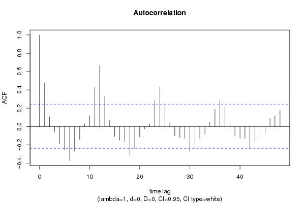
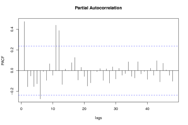
Title produced by software

(Partial) Autocorrelation Function

Date of computation

Sat, 11 Dec 2010 12:03:59 +0000

Cite this page as follows

Statistical Computations at FreeStatistics.org, Office for Research Development and Education, URL https://freestatistics.org/blog/index.php?v=date/2010/Dec/11/t1292068915rnp8vtaxrt1lt7m.htm/, Retrieved Mon, 06 May 2024 13:45:31 +0000

Statistical Computations at FreeStatistics.org, Office for Research Development and Education, URL https://freestatistics.org/blog/index.php?pk=108079, Retrieved Mon, 06 May 2024 13:45:31 +0000

QR Codes:

Paste this QR Code to cite your computation.

Original text written by user:

IsPrivate?

No (this computation is public)

User-defined keywords

Estimated Impact

143

Family? (F = Feedback message, R = changed R code, M = changed R Module, P = changed Parameters, D = changed Data)

-     [Univariate Explorative Data Analysis] [paper] [2007-12-11 21:01:08] [b3bb3ec527e23fa7d74d4348b38c8499]
- RMPD  [Univariate Explorative Data Analysis] [PAPER] [2009-12-30 15:50:30] [23722951c28e05bb35cc9a97084fe0d9]
- RMPD      [(Partial) Autocorrelation Function] [Paper ACF] [2010-12-11 12:03:59] [81b44bf7e2a3251743773b0d7e91dd87] [Current]
-             [(Partial) Autocorrelation Function] [Paper ACF 2] [2010-12-11 13:24:27] [6e6854a111a7f2438dd668bfaa6f3aa0] 
- RM          [Variance Reduction Matrix] [Paper VRM] [2010-12-11 13:35:00] [6e6854a111a7f2438dd668bfaa6f3aa0] 
- RM          [Spectral Analysis] [Paper Spectraal] [2010-12-11 13:44:53] [6e6854a111a7f2438dd668bfaa6f3aa0] 
- RM            [ARIMA Backward Selection] [Paper Arima backward] [2010-12-11 14:34:06] [6e6854a111a7f2438dd668bfaa6f3aa0] 
- RM D          [Central Tendency] [Paper robustness ...] [2010-12-11 14:54:55] [6e6854a111a7f2438dd668bfaa6f3aa0] 

Feedback Forum

Post a new message

Dataseries X:

Download CSV

Histogram

Boxplots

Summary of computational transaction
Raw Input	view raw input (R code)
Raw Output	view raw output of R engine
Computing time	1 seconds
R Server	'Gwilym Jenkins' @ 72.249.127.135

\begin{tabular}{lllllllll}
\hline
Summary of computational transaction \tabularnewline
Raw Input & view raw input (R code)  \tabularnewline
Raw Output & view raw output of R engine  \tabularnewline
Computing time & 1 seconds \tabularnewline
R Server & 'Gwilym Jenkins' @ 72.249.127.135 \tabularnewline
\hline
\end{tabular}
%Source: https://freestatistics.org/blog/index.php?pk=108079&T=0

[TABLE]
[ROW][C]Summary of computational transaction[/C][/ROW]
[ROW][C]Raw Input[/C][C]view raw input (R code) [/C][/ROW]
[ROW][C]Raw Output[/C][C]view raw output of R engine [/C][/ROW]
[ROW][C]Computing time[/C][C]1 seconds[/C][/ROW]
[ROW][C]R Server[/C][C]'Gwilym Jenkins' @ 72.249.127.135[/C][/ROW]
[/TABLE]
Source: https://freestatistics.org/blog/index.php?pk=108079&T=0

Globally Unique Identifier (entire table): ba.freestatistics.org/blog/index.php?pk=108079&T=0

As an alternative you can also use a QR Code:

The GUIDs for individual cells are displayed in the table below:

Summary of computational transaction
Raw Input	view raw input (R code)
Raw Output	view raw output of R engine
Computing time	1 seconds
R Server	'Gwilym Jenkins' @ 72.249.127.135

Autocorrelation Function
Time lag k	ACF(k)	T-STAT	P-value
1	0.475778	3.9234	0.000103
2	0.10483	0.8645	0.19519
3	-0.056481	-0.4658	0.321439
4	-0.185679	-1.5311	0.065186
5	-0.255376	-2.1059	0.019455
6	-0.373751	-3.082	0.001484
7	-0.267055	-2.2022	0.015523
8	-0.141644	-1.168	0.123438
9	0.029985	0.2473	0.402726
10	0.118227	0.9749	0.166526
11	0.428691	3.5351	0.000369
12	0.66513	5.4848	0
13	0.329426	2.7165	0.004179
14	0.066256	0.5464	0.293302
15	-0.110116	-0.908	0.183531
16	-0.149777	-1.2351	0.110523
17	-0.163599	-1.3491	0.090894
18	-0.314024	-2.5895	0.005873
19	-0.242027	-1.9958	0.024981
20	-0.115195	-0.9499	0.172758
21	-0.030136	-0.2485	0.402245
22	0.027714	0.2285	0.409959
23	0.283718	2.3396	0.011124
24	0.433933	3.5783	0.000322
25	0.259604	2.1408	0.017941
26	0.041672	0.3436	0.36609
27	-0.103293	-0.8518	0.198665
28	-0.120607	-0.9945	0.161741
29	-0.127005	-1.0473	0.149332
30	-0.27912	-2.3017	0.012211
31	-0.237371	-1.9574	0.027202
32	-0.134933	-1.1127	0.13488
33	-0.08879	-0.7322	0.233287
34	0.046791	0.3858	0.350406
35	0.190749	1.573	0.060185
36	0.283643	2.339	0.011141
37	0.222177	1.8321	0.035657
38	0.040366	0.3329	0.370129
39	-0.10027	-0.8269	0.205607
40	-0.128136	-1.0566	0.147208
41	-0.128273	-1.0578	0.146954
42	-0.248939	-2.0528	0.021971
43	-0.167514	-1.3814	0.085846
44	-0.13354	-1.1012	0.137347
45	-0.070849	-0.5842	0.280497
46	0.092881	0.7659	0.223188
47	0.116251	0.9586	0.17057
48	0.177794	1.4661	0.073611

\begin{tabular}{lllllllll}
\hline
Autocorrelation Function \tabularnewline
Time lag k & ACF(k) & T-STAT & P-value \tabularnewline
1 & 0.475778 & 3.9234 & 0.000103 \tabularnewline
2 & 0.10483 & 0.8645 & 0.19519 \tabularnewline
3 & -0.056481 & -0.4658 & 0.321439 \tabularnewline
4 & -0.185679 & -1.5311 & 0.065186 \tabularnewline
5 & -0.255376 & -2.1059 & 0.019455 \tabularnewline
6 & -0.373751 & -3.082 & 0.001484 \tabularnewline
7 & -0.267055 & -2.2022 & 0.015523 \tabularnewline
8 & -0.141644 & -1.168 & 0.123438 \tabularnewline
9 & 0.029985 & 0.2473 & 0.402726 \tabularnewline
10 & 0.118227 & 0.9749 & 0.166526 \tabularnewline
11 & 0.428691 & 3.5351 & 0.000369 \tabularnewline
12 & 0.66513 & 5.4848 & 0 \tabularnewline
13 & 0.329426 & 2.7165 & 0.004179 \tabularnewline
14 & 0.066256 & 0.5464 & 0.293302 \tabularnewline
15 & -0.110116 & -0.908 & 0.183531 \tabularnewline
16 & -0.149777 & -1.2351 & 0.110523 \tabularnewline
17 & -0.163599 & -1.3491 & 0.090894 \tabularnewline
18 & -0.314024 & -2.5895 & 0.005873 \tabularnewline
19 & -0.242027 & -1.9958 & 0.024981 \tabularnewline
20 & -0.115195 & -0.9499 & 0.172758 \tabularnewline
21 & -0.030136 & -0.2485 & 0.402245 \tabularnewline
22 & 0.027714 & 0.2285 & 0.409959 \tabularnewline
23 & 0.283718 & 2.3396 & 0.011124 \tabularnewline
24 & 0.433933 & 3.5783 & 0.000322 \tabularnewline
25 & 0.259604 & 2.1408 & 0.017941 \tabularnewline
26 & 0.041672 & 0.3436 & 0.36609 \tabularnewline
27 & -0.103293 & -0.8518 & 0.198665 \tabularnewline
28 & -0.120607 & -0.9945 & 0.161741 \tabularnewline
29 & -0.127005 & -1.0473 & 0.149332 \tabularnewline
30 & -0.27912 & -2.3017 & 0.012211 \tabularnewline
31 & -0.237371 & -1.9574 & 0.027202 \tabularnewline
32 & -0.134933 & -1.1127 & 0.13488 \tabularnewline
33 & -0.08879 & -0.7322 & 0.233287 \tabularnewline
34 & 0.046791 & 0.3858 & 0.350406 \tabularnewline
35 & 0.190749 & 1.573 & 0.060185 \tabularnewline
36 & 0.283643 & 2.339 & 0.011141 \tabularnewline
37 & 0.222177 & 1.8321 & 0.035657 \tabularnewline
38 & 0.040366 & 0.3329 & 0.370129 \tabularnewline
39 & -0.10027 & -0.8269 & 0.205607 \tabularnewline
40 & -0.128136 & -1.0566 & 0.147208 \tabularnewline
41 & -0.128273 & -1.0578 & 0.146954 \tabularnewline
42 & -0.248939 & -2.0528 & 0.021971 \tabularnewline
43 & -0.167514 & -1.3814 & 0.085846 \tabularnewline
44 & -0.13354 & -1.1012 & 0.137347 \tabularnewline
45 & -0.070849 & -0.5842 & 0.280497 \tabularnewline
46 & 0.092881 & 0.7659 & 0.223188 \tabularnewline
47 & 0.116251 & 0.9586 & 0.17057 \tabularnewline
48 & 0.177794 & 1.4661 & 0.073611 \tabularnewline
\hline
\end{tabular}
%Source: https://freestatistics.org/blog/index.php?pk=108079&T=1

[TABLE]
[ROW][C]Autocorrelation Function[/C][/ROW]
[ROW][C]Time lag k[/C][C]ACF(k)[/C][C]T-STAT[/C][C]P-value[/C][/ROW]
[ROW][C]1[/C][C]0.475778[/C][C]3.9234[/C][C]0.000103[/C][/ROW]
[ROW][C]2[/C][C]0.10483[/C][C]0.8645[/C][C]0.19519[/C][/ROW]
[ROW][C]3[/C][C]-0.056481[/C][C]-0.4658[/C][C]0.321439[/C][/ROW]
[ROW][C]4[/C][C]-0.185679[/C][C]-1.5311[/C][C]0.065186[/C][/ROW]
[ROW][C]5[/C][C]-0.255376[/C][C]-2.1059[/C][C]0.019455[/C][/ROW]
[ROW][C]6[/C][C]-0.373751[/C][C]-3.082[/C][C]0.001484[/C][/ROW]
[ROW][C]7[/C][C]-0.267055[/C][C]-2.2022[/C][C]0.015523[/C][/ROW]
[ROW][C]8[/C][C]-0.141644[/C][C]-1.168[/C][C]0.123438[/C][/ROW]
[ROW][C]9[/C][C]0.029985[/C][C]0.2473[/C][C]0.402726[/C][/ROW]
[ROW][C]10[/C][C]0.118227[/C][C]0.9749[/C][C]0.166526[/C][/ROW]
[ROW][C]11[/C][C]0.428691[/C][C]3.5351[/C][C]0.000369[/C][/ROW]
[ROW][C]12[/C][C]0.66513[/C][C]5.4848[/C][C]0[/C][/ROW]
[ROW][C]13[/C][C]0.329426[/C][C]2.7165[/C][C]0.004179[/C][/ROW]
[ROW][C]14[/C][C]0.066256[/C][C]0.5464[/C][C]0.293302[/C][/ROW]
[ROW][C]15[/C][C]-0.110116[/C][C]-0.908[/C][C]0.183531[/C][/ROW]
[ROW][C]16[/C][C]-0.149777[/C][C]-1.2351[/C][C]0.110523[/C][/ROW]
[ROW][C]17[/C][C]-0.163599[/C][C]-1.3491[/C][C]0.090894[/C][/ROW]
[ROW][C]18[/C][C]-0.314024[/C][C]-2.5895[/C][C]0.005873[/C][/ROW]
[ROW][C]19[/C][C]-0.242027[/C][C]-1.9958[/C][C]0.024981[/C][/ROW]
[ROW][C]20[/C][C]-0.115195[/C][C]-0.9499[/C][C]0.172758[/C][/ROW]
[ROW][C]21[/C][C]-0.030136[/C][C]-0.2485[/C][C]0.402245[/C][/ROW]
[ROW][C]22[/C][C]0.027714[/C][C]0.2285[/C][C]0.409959[/C][/ROW]
[ROW][C]23[/C][C]0.283718[/C][C]2.3396[/C][C]0.011124[/C][/ROW]
[ROW][C]24[/C][C]0.433933[/C][C]3.5783[/C][C]0.000322[/C][/ROW]
[ROW][C]25[/C][C]0.259604[/C][C]2.1408[/C][C]0.017941[/C][/ROW]
[ROW][C]26[/C][C]0.041672[/C][C]0.3436[/C][C]0.36609[/C][/ROW]
[ROW][C]27[/C][C]-0.103293[/C][C]-0.8518[/C][C]0.198665[/C][/ROW]
[ROW][C]28[/C][C]-0.120607[/C][C]-0.9945[/C][C]0.161741[/C][/ROW]
[ROW][C]29[/C][C]-0.127005[/C][C]-1.0473[/C][C]0.149332[/C][/ROW]
[ROW][C]30[/C][C]-0.27912[/C][C]-2.3017[/C][C]0.012211[/C][/ROW]
[ROW][C]31[/C][C]-0.237371[/C][C]-1.9574[/C][C]0.027202[/C][/ROW]
[ROW][C]32[/C][C]-0.134933[/C][C]-1.1127[/C][C]0.13488[/C][/ROW]
[ROW][C]33[/C][C]-0.08879[/C][C]-0.7322[/C][C]0.233287[/C][/ROW]
[ROW][C]34[/C][C]0.046791[/C][C]0.3858[/C][C]0.350406[/C][/ROW]
[ROW][C]35[/C][C]0.190749[/C][C]1.573[/C][C]0.060185[/C][/ROW]
[ROW][C]36[/C][C]0.283643[/C][C]2.339[/C][C]0.011141[/C][/ROW]
[ROW][C]37[/C][C]0.222177[/C][C]1.8321[/C][C]0.035657[/C][/ROW]
[ROW][C]38[/C][C]0.040366[/C][C]0.3329[/C][C]0.370129[/C][/ROW]
[ROW][C]39[/C][C]-0.10027[/C][C]-0.8269[/C][C]0.205607[/C][/ROW]
[ROW][C]40[/C][C]-0.128136[/C][C]-1.0566[/C][C]0.147208[/C][/ROW]
[ROW][C]41[/C][C]-0.128273[/C][C]-1.0578[/C][C]0.146954[/C][/ROW]
[ROW][C]42[/C][C]-0.248939[/C][C]-2.0528[/C][C]0.021971[/C][/ROW]
[ROW][C]43[/C][C]-0.167514[/C][C]-1.3814[/C][C]0.085846[/C][/ROW]
[ROW][C]44[/C][C]-0.13354[/C][C]-1.1012[/C][C]0.137347[/C][/ROW]
[ROW][C]45[/C][C]-0.070849[/C][C]-0.5842[/C][C]0.280497[/C][/ROW]
[ROW][C]46[/C][C]0.092881[/C][C]0.7659[/C][C]0.223188[/C][/ROW]
[ROW][C]47[/C][C]0.116251[/C][C]0.9586[/C][C]0.17057[/C][/ROW]
[ROW][C]48[/C][C]0.177794[/C][C]1.4661[/C][C]0.073611[/C][/ROW]
[/TABLE]
Source: https://freestatistics.org/blog/index.php?pk=108079&T=1

Globally Unique Identifier (entire table): ba.freestatistics.org/blog/index.php?pk=108079&T=1

As an alternative you can also use a QR Code:

The GUIDs for individual cells are displayed in the table below:

Autocorrelation Function
Time lag k	ACF(k)	T-STAT	P-value
1	0.475778	3.9234	0.000103
2	0.10483	0.8645	0.19519
3	-0.056481	-0.4658	0.321439
4	-0.185679	-1.5311	0.065186
5	-0.255376	-2.1059	0.019455
6	-0.373751	-3.082	0.001484
7	-0.267055	-2.2022	0.015523
8	-0.141644	-1.168	0.123438
9	0.029985	0.2473	0.402726
10	0.118227	0.9749	0.166526
11	0.428691	3.5351	0.000369
12	0.66513	5.4848	0
13	0.329426	2.7165	0.004179
14	0.066256	0.5464	0.293302
15	-0.110116	-0.908	0.183531
16	-0.149777	-1.2351	0.110523
17	-0.163599	-1.3491	0.090894
18	-0.314024	-2.5895	0.005873
19	-0.242027	-1.9958	0.024981
20	-0.115195	-0.9499	0.172758
21	-0.030136	-0.2485	0.402245
22	0.027714	0.2285	0.409959
23	0.283718	2.3396	0.011124
24	0.433933	3.5783	0.000322
25	0.259604	2.1408	0.017941
26	0.041672	0.3436	0.36609
27	-0.103293	-0.8518	0.198665
28	-0.120607	-0.9945	0.161741
29	-0.127005	-1.0473	0.149332
30	-0.27912	-2.3017	0.012211
31	-0.237371	-1.9574	0.027202
32	-0.134933	-1.1127	0.13488
33	-0.08879	-0.7322	0.233287
34	0.046791	0.3858	0.350406
35	0.190749	1.573	0.060185
36	0.283643	2.339	0.011141
37	0.222177	1.8321	0.035657
38	0.040366	0.3329	0.370129
39	-0.10027	-0.8269	0.205607
40	-0.128136	-1.0566	0.147208
41	-0.128273	-1.0578	0.146954
42	-0.248939	-2.0528	0.021971
43	-0.167514	-1.3814	0.085846
44	-0.13354	-1.1012	0.137347
45	-0.070849	-0.5842	0.280497
46	0.092881	0.7659	0.223188
47	0.116251	0.9586	0.17057
48	0.177794	1.4661	0.073611

Partial Autocorrelation Function
Time lag k	PACF(k)	T-STAT	P-value
1	0.475778	3.9234	0.000103
2	-0.157096	-1.2954	0.099774
3	-0.052283	-0.4311	0.333866
4	-0.155118	-1.2791	0.102599
5	-0.128129	-1.0566	0.147222
6	-0.274667	-2.265	0.013353
7	-0.00847	-0.0698	0.472262
8	-0.095073	-0.784	0.217883
9	0.066812	0.5509	0.291739
10	-0.045264	-0.3733	0.355059
11	0.440984	3.6364	0.000267
12	0.388598	3.2045	0.001031
13	-0.134806	-1.1116	0.135105
14	0.015315	0.1263	0.449937
15	-0.000325	-0.0027	0.498936
16	0.07741	0.6383	0.262698
17	0.127642	1.0526	0.148134
18	-0.091342	-0.7532	0.226958
19	0.032327	0.2666	0.3953
20	-0.056457	-0.4656	0.321509
21	-0.149969	-1.2367	0.110231
22	-0.118613	-0.9781	0.165744
23	-0.000765	-0.0063	0.497493
24	-0.010751	-0.0887	0.46481
25	0.020108	0.1658	0.434396
26	-0.094757	-0.7814	0.218643
27	0.01783	0.147	0.441772
28	-0.121414	-1.0012	0.160138
29	0.037079	0.3058	0.380359
30	-0.080836	-0.6666	0.253646
31	0.022797	0.188	0.425723
32	-0.044967	-0.3708	0.355968
33	-0.028745	-0.237	0.406672
34	0.085475	0.7048	0.241656
35	-0.056108	-0.4627	0.322536
36	-0.071736	-0.5916	0.278056
37	0.08658	0.714	0.238848
38	-0.031956	-0.2635	0.396474
39	-0.008031	-0.0662	0.473695
40	-0.085162	-0.7023	0.242455
41	0.023678	0.1953	0.422887
42	-0.045245	-0.3731	0.355118
43	0.096505	0.7958	0.214459
44	-0.109363	-0.9018	0.185165
45	0.071928	0.5931	0.27753
46	0.006441	0.0531	0.478898
47	-0.045488	-0.3751	0.354376
48	-0.103428	-0.8529	0.198357

\begin{tabular}{lllllllll}
\hline
Partial Autocorrelation Function \tabularnewline
Time lag k & PACF(k) & T-STAT & P-value \tabularnewline
1 & 0.475778 & 3.9234 & 0.000103 \tabularnewline
2 & -0.157096 & -1.2954 & 0.099774 \tabularnewline
3 & -0.052283 & -0.4311 & 0.333866 \tabularnewline
4 & -0.155118 & -1.2791 & 0.102599 \tabularnewline
5 & -0.128129 & -1.0566 & 0.147222 \tabularnewline
6 & -0.274667 & -2.265 & 0.013353 \tabularnewline
7 & -0.00847 & -0.0698 & 0.472262 \tabularnewline
8 & -0.095073 & -0.784 & 0.217883 \tabularnewline
9 & 0.066812 & 0.5509 & 0.291739 \tabularnewline
10 & -0.045264 & -0.3733 & 0.355059 \tabularnewline
11 & 0.440984 & 3.6364 & 0.000267 \tabularnewline
12 & 0.388598 & 3.2045 & 0.001031 \tabularnewline
13 & -0.134806 & -1.1116 & 0.135105 \tabularnewline
14 & 0.015315 & 0.1263 & 0.449937 \tabularnewline
15 & -0.000325 & -0.0027 & 0.498936 \tabularnewline
16 & 0.07741 & 0.6383 & 0.262698 \tabularnewline
17 & 0.127642 & 1.0526 & 0.148134 \tabularnewline
18 & -0.091342 & -0.7532 & 0.226958 \tabularnewline
19 & 0.032327 & 0.2666 & 0.3953 \tabularnewline
20 & -0.056457 & -0.4656 & 0.321509 \tabularnewline
21 & -0.149969 & -1.2367 & 0.110231 \tabularnewline
22 & -0.118613 & -0.9781 & 0.165744 \tabularnewline
23 & -0.000765 & -0.0063 & 0.497493 \tabularnewline
24 & -0.010751 & -0.0887 & 0.46481 \tabularnewline
25 & 0.020108 & 0.1658 & 0.434396 \tabularnewline
26 & -0.094757 & -0.7814 & 0.218643 \tabularnewline
27 & 0.01783 & 0.147 & 0.441772 \tabularnewline
28 & -0.121414 & -1.0012 & 0.160138 \tabularnewline
29 & 0.037079 & 0.3058 & 0.380359 \tabularnewline
30 & -0.080836 & -0.6666 & 0.253646 \tabularnewline
31 & 0.022797 & 0.188 & 0.425723 \tabularnewline
32 & -0.044967 & -0.3708 & 0.355968 \tabularnewline
33 & -0.028745 & -0.237 & 0.406672 \tabularnewline
34 & 0.085475 & 0.7048 & 0.241656 \tabularnewline
35 & -0.056108 & -0.4627 & 0.322536 \tabularnewline
36 & -0.071736 & -0.5916 & 0.278056 \tabularnewline
37 & 0.08658 & 0.714 & 0.238848 \tabularnewline
38 & -0.031956 & -0.2635 & 0.396474 \tabularnewline
39 & -0.008031 & -0.0662 & 0.473695 \tabularnewline
40 & -0.085162 & -0.7023 & 0.242455 \tabularnewline
41 & 0.023678 & 0.1953 & 0.422887 \tabularnewline
42 & -0.045245 & -0.3731 & 0.355118 \tabularnewline
43 & 0.096505 & 0.7958 & 0.214459 \tabularnewline
44 & -0.109363 & -0.9018 & 0.185165 \tabularnewline
45 & 0.071928 & 0.5931 & 0.27753 \tabularnewline
46 & 0.006441 & 0.0531 & 0.478898 \tabularnewline
47 & -0.045488 & -0.3751 & 0.354376 \tabularnewline
48 & -0.103428 & -0.8529 & 0.198357 \tabularnewline
\hline
\end{tabular}
%Source: https://freestatistics.org/blog/index.php?pk=108079&T=2

[TABLE]
[ROW][C]Partial Autocorrelation Function[/C][/ROW]
[ROW][C]Time lag k[/C][C]PACF(k)[/C][C]T-STAT[/C][C]P-value[/C][/ROW]
[ROW][C]1[/C][C]0.475778[/C][C]3.9234[/C][C]0.000103[/C][/ROW]
[ROW][C]2[/C][C]-0.157096[/C][C]-1.2954[/C][C]0.099774[/C][/ROW]
[ROW][C]3[/C][C]-0.052283[/C][C]-0.4311[/C][C]0.333866[/C][/ROW]
[ROW][C]4[/C][C]-0.155118[/C][C]-1.2791[/C][C]0.102599[/C][/ROW]
[ROW][C]5[/C][C]-0.128129[/C][C]-1.0566[/C][C]0.147222[/C][/ROW]
[ROW][C]6[/C][C]-0.274667[/C][C]-2.265[/C][C]0.013353[/C][/ROW]
[ROW][C]7[/C][C]-0.00847[/C][C]-0.0698[/C][C]0.472262[/C][/ROW]
[ROW][C]8[/C][C]-0.095073[/C][C]-0.784[/C][C]0.217883[/C][/ROW]
[ROW][C]9[/C][C]0.066812[/C][C]0.5509[/C][C]0.291739[/C][/ROW]
[ROW][C]10[/C][C]-0.045264[/C][C]-0.3733[/C][C]0.355059[/C][/ROW]
[ROW][C]11[/C][C]0.440984[/C][C]3.6364[/C][C]0.000267[/C][/ROW]
[ROW][C]12[/C][C]0.388598[/C][C]3.2045[/C][C]0.001031[/C][/ROW]
[ROW][C]13[/C][C]-0.134806[/C][C]-1.1116[/C][C]0.135105[/C][/ROW]
[ROW][C]14[/C][C]0.015315[/C][C]0.1263[/C][C]0.449937[/C][/ROW]
[ROW][C]15[/C][C]-0.000325[/C][C]-0.0027[/C][C]0.498936[/C][/ROW]
[ROW][C]16[/C][C]0.07741[/C][C]0.6383[/C][C]0.262698[/C][/ROW]
[ROW][C]17[/C][C]0.127642[/C][C]1.0526[/C][C]0.148134[/C][/ROW]
[ROW][C]18[/C][C]-0.091342[/C][C]-0.7532[/C][C]0.226958[/C][/ROW]
[ROW][C]19[/C][C]0.032327[/C][C]0.2666[/C][C]0.3953[/C][/ROW]
[ROW][C]20[/C][C]-0.056457[/C][C]-0.4656[/C][C]0.321509[/C][/ROW]
[ROW][C]21[/C][C]-0.149969[/C][C]-1.2367[/C][C]0.110231[/C][/ROW]
[ROW][C]22[/C][C]-0.118613[/C][C]-0.9781[/C][C]0.165744[/C][/ROW]
[ROW][C]23[/C][C]-0.000765[/C][C]-0.0063[/C][C]0.497493[/C][/ROW]
[ROW][C]24[/C][C]-0.010751[/C][C]-0.0887[/C][C]0.46481[/C][/ROW]
[ROW][C]25[/C][C]0.020108[/C][C]0.1658[/C][C]0.434396[/C][/ROW]
[ROW][C]26[/C][C]-0.094757[/C][C]-0.7814[/C][C]0.218643[/C][/ROW]
[ROW][C]27[/C][C]0.01783[/C][C]0.147[/C][C]0.441772[/C][/ROW]
[ROW][C]28[/C][C]-0.121414[/C][C]-1.0012[/C][C]0.160138[/C][/ROW]
[ROW][C]29[/C][C]0.037079[/C][C]0.3058[/C][C]0.380359[/C][/ROW]
[ROW][C]30[/C][C]-0.080836[/C][C]-0.6666[/C][C]0.253646[/C][/ROW]
[ROW][C]31[/C][C]0.022797[/C][C]0.188[/C][C]0.425723[/C][/ROW]
[ROW][C]32[/C][C]-0.044967[/C][C]-0.3708[/C][C]0.355968[/C][/ROW]
[ROW][C]33[/C][C]-0.028745[/C][C]-0.237[/C][C]0.406672[/C][/ROW]
[ROW][C]34[/C][C]0.085475[/C][C]0.7048[/C][C]0.241656[/C][/ROW]
[ROW][C]35[/C][C]-0.056108[/C][C]-0.4627[/C][C]0.322536[/C][/ROW]
[ROW][C]36[/C][C]-0.071736[/C][C]-0.5916[/C][C]0.278056[/C][/ROW]
[ROW][C]37[/C][C]0.08658[/C][C]0.714[/C][C]0.238848[/C][/ROW]
[ROW][C]38[/C][C]-0.031956[/C][C]-0.2635[/C][C]0.396474[/C][/ROW]
[ROW][C]39[/C][C]-0.008031[/C][C]-0.0662[/C][C]0.473695[/C][/ROW]
[ROW][C]40[/C][C]-0.085162[/C][C]-0.7023[/C][C]0.242455[/C][/ROW]
[ROW][C]41[/C][C]0.023678[/C][C]0.1953[/C][C]0.422887[/C][/ROW]
[ROW][C]42[/C][C]-0.045245[/C][C]-0.3731[/C][C]0.355118[/C][/ROW]
[ROW][C]43[/C][C]0.096505[/C][C]0.7958[/C][C]0.214459[/C][/ROW]
[ROW][C]44[/C][C]-0.109363[/C][C]-0.9018[/C][C]0.185165[/C][/ROW]
[ROW][C]45[/C][C]0.071928[/C][C]0.5931[/C][C]0.27753[/C][/ROW]
[ROW][C]46[/C][C]0.006441[/C][C]0.0531[/C][C]0.478898[/C][/ROW]
[ROW][C]47[/C][C]-0.045488[/C][C]-0.3751[/C][C]0.354376[/C][/ROW]
[ROW][C]48[/C][C]-0.103428[/C][C]-0.8529[/C][C]0.198357[/C][/ROW]
[/TABLE]
Source: https://freestatistics.org/blog/index.php?pk=108079&T=2

Globally Unique Identifier (entire table): ba.freestatistics.org/blog/index.php?pk=108079&T=2

As an alternative you can also use a QR Code:

The GUIDs for individual cells are displayed in the table below:

Partial Autocorrelation Function
Time lag k	PACF(k)	T-STAT	P-value
1	0.475778	3.9234	0.000103
2	-0.157096	-1.2954	0.099774
3	-0.052283	-0.4311	0.333866
4	-0.155118	-1.2791	0.102599
5	-0.128129	-1.0566	0.147222
6	-0.274667	-2.265	0.013353
7	-0.00847	-0.0698	0.472262
8	-0.095073	-0.784	0.217883
9	0.066812	0.5509	0.291739
10	-0.045264	-0.3733	0.355059
11	0.440984	3.6364	0.000267
12	0.388598	3.2045	0.001031
13	-0.134806	-1.1116	0.135105
14	0.015315	0.1263	0.449937
15	-0.000325	-0.0027	0.498936
16	0.07741	0.6383	0.262698
17	0.127642	1.0526	0.148134
18	-0.091342	-0.7532	0.226958
19	0.032327	0.2666	0.3953
20	-0.056457	-0.4656	0.321509
21	-0.149969	-1.2367	0.110231
22	-0.118613	-0.9781	0.165744
23	-0.000765	-0.0063	0.497493
24	-0.010751	-0.0887	0.46481
25	0.020108	0.1658	0.434396
26	-0.094757	-0.7814	0.218643
27	0.01783	0.147	0.441772
28	-0.121414	-1.0012	0.160138
29	0.037079	0.3058	0.380359
30	-0.080836	-0.6666	0.253646
31	0.022797	0.188	0.425723
32	-0.044967	-0.3708	0.355968
33	-0.028745	-0.237	0.406672
34	0.085475	0.7048	0.241656
35	-0.056108	-0.4627	0.322536
36	-0.071736	-0.5916	0.278056
37	0.08658	0.714	0.238848
38	-0.031956	-0.2635	0.396474
39	-0.008031	-0.0662	0.473695
40	-0.085162	-0.7023	0.242455
41	0.023678	0.1953	0.422887
42	-0.045245	-0.3731	0.355118
43	0.096505	0.7958	0.214459
44	-0.109363	-0.9018	0.185165
45	0.071928	0.5931	0.27753
46	0.006441	0.0531	0.478898
47	-0.045488	-0.3751	0.354376
48	-0.103428	-0.8529	0.198357

Figure 1

PNG link

Postscript link

PDF link

Figure 2

PNG link

Postscript link

PDF link

Parameters (Session):

Parameters (R input):

par1 = 48 ; par2 = 1 ; par3 = 0 ; par4 = 0 ; par5 = 12 ; par6 = White Noise ; par7 = 0.95 ;

R code (references can be found in the software module):

if (par1 == 'Default') {
par1 = 10*log10(length(x))
} else {
par1 <- as.numeric(par1)
}
par2 <- as.numeric(par2)
par3 <- as.numeric(par3)
par4 <- as.numeric(par4)
par5 <- as.numeric(par5)
if (par6 == 'White Noise') par6 <- 'white' else par6 <- 'ma'
par7 <- as.numeric(par7)
if (par2 == 0) {
x <- log(x)
} else {
x <- (x ^ par2 - 1) / par2
}
if (par3 > 0) x <- diff(x,lag=1,difference=par3)
if (par4 > 0) x <- diff(x,lag=par5,difference=par4)
bitmap(file='pic1.png')
racf <- acf(x, par1, main='Autocorrelation', xlab='time lag', ylab='ACF', ci.type=par6, ci=par7, sub=paste('(lambda=',par2,', d=',par3,', D=',par4,', CI=', par7, ', CI type=',par6,')',sep=''))
dev.off()
bitmap(file='pic2.png')
rpacf <- pacf(x,par1,main='Partial Autocorrelation',xlab='lags',ylab='PACF')
dev.off()
(myacf <- c(racf$acf))
(mypacf <- c(rpacf$acf))
lengthx <- length(x)
sqrtn <- sqrt(lengthx)
load(file='createtable')
a<-table.start()
a<-table.row.start(a)
a<-table.element(a,'Autocorrelation Function',4,TRUE)
a<-table.row.end(a)
a<-table.row.start(a)
a<-table.element(a,'Time lag k',header=TRUE)
a<-table.element(a,hyperlink('basics.htm','ACF(k)','click here for more information about the Autocorrelation Function'),header=TRUE)
a<-table.element(a,'T-STAT',header=TRUE)
a<-table.element(a,'P-value',header=TRUE)
a<-table.row.end(a)
for (i in 2:(par1+1)) {
a<-table.row.start(a)
a<-table.element(a,i-1,header=TRUE)
a<-table.element(a,round(myacf[i],6))
mytstat <- myacf[i]*sqrtn
a<-table.element(a,round(mytstat,4))
a<-table.element(a,round(1-pt(abs(mytstat),lengthx),6))
a<-table.row.end(a)
}
a<-table.end(a)
table.save(a,file='mytable.tab')
a<-table.start()
a<-table.row.start(a)
a<-table.element(a,'Partial Autocorrelation Function',4,TRUE)
a<-table.row.end(a)
a<-table.row.start(a)
a<-table.element(a,'Time lag k',header=TRUE)
a<-table.element(a,hyperlink('basics.htm','PACF(k)','click here for more information about the Partial Autocorrelation Function'),header=TRUE)
a<-table.element(a,'T-STAT',header=TRUE)
a<-table.element(a,'P-value',header=TRUE)
a<-table.row.end(a)
for (i in 1:par1) {
a<-table.row.start(a)
a<-table.element(a,i,header=TRUE)
a<-table.element(a,round(mypacf[i],6))
mytstat <- mypacf[i]*sqrtn
a<-table.element(a,round(mytstat,4))
a<-table.element(a,round(1-pt(abs(mytstat),lengthx),6))
a<-table.row.end(a)
}
a<-table.end(a)
table.save(a,file='mytable1.tab')

Free Statistics

Description of Statistical Computation

Tree of Dependent Computations

Dataset

Tables (Output of Computation)

Figures (Output of Computation)

Input Parameters & R Code