Repository of Reproducible Computations

Free Statistics

of Irreproducible Research!

Author's title

Author

*Unverified author*

R Software Module

rwasp_autocorrelation.wasp

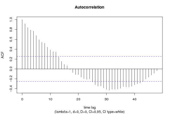
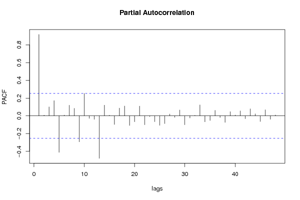
Title produced by software

(Partial) Autocorrelation Function

Date of computation

Fri, 10 Dec 2010 19:48:20 +0000

Cite this page as follows

Statistical Computations at FreeStatistics.org, Office for Research Development and Education, URL https://freestatistics.org/blog/index.php?v=date/2010/Dec/10/t12920104599o7dyqnh29d14m1.htm/, Retrieved Mon, 29 Apr 2024 13:15:50 +0000

Statistical Computations at FreeStatistics.org, Office for Research Development and Education, URL https://freestatistics.org/blog/index.php?pk=107913, Retrieved Mon, 29 Apr 2024 13:15:50 +0000

QR Codes:

Paste this QR Code to cite your computation.

Original text written by user:

IsPrivate?

No (this computation is public)

User-defined keywords

Estimated Impact

100

Family? (F = Feedback message, R = changed R code, M = changed R Module, P = changed Parameters, D = changed Data)

-     [Univariate Explorative Data Analysis] [Run Sequence gebo...] [2008-12-12 13:32:37] [76963dc1903f0f612b6153510a3818cf]
- R  D  [Univariate Explorative Data Analysis] [Run Sequence gebo...] [2008-12-17 12:14:40] [76963dc1903f0f612b6153510a3818cf]
-         [Univariate Explorative Data Analysis] [Run Sequence Plot...] [2008-12-22 18:19:51] [1ce0d16c8f4225c977b42c8fa93bc163]
- RMP       [Univariate Data Series] [Identifying Integ...] [2009-11-22 12:08:06] [b98453cac15ba1066b407e146608df68]
- RMP         [(Partial) Autocorrelation Function] [Births] [2010-11-29 09:36:27] [b98453cac15ba1066b407e146608df68]
-   PD            [(Partial) Autocorrelation Function] [Workshop 9] [2010-12-10 19:48:20] [d41d8cd98f00b204e9800998ecf8427e] [Current]
-   P               [(Partial) Autocorrelation Function] [Workshop 9] [2010-12-10 20:02:02] [74be16979710d4c4e7c6647856088456] 
-   P                 [(Partial) Autocorrelation Function] [Workshop 9] [2010-12-10 20:21:41] [74be16979710d4c4e7c6647856088456] 
-   P                   [(Partial) Autocorrelation Function] [] [2010-12-10 21:12:03] [1ec36cc0fd92fd0f07d0b885ce2c369b] 
-   P                 [(Partial) Autocorrelation Function] [] [2010-12-10 21:12:45] [1ec36cc0fd92fd0f07d0b885ce2c369b] 
-   P               [(Partial) Autocorrelation Function] [] [2010-12-10 21:13:21] [1ec36cc0fd92fd0f07d0b885ce2c369b] 

Feedback Forum

Post a new message

Dataseries X:

Download CSV

Histogram

Boxplots

Summary of computational transaction
Raw Input	view raw input (R code)
Raw Output	view raw output of R engine
Computing time	4 seconds
R Server	'Gwilym Jenkins' @ 72.249.127.135

\begin{tabular}{lllllllll}
\hline
Summary of computational transaction \tabularnewline
Raw Input & view raw input (R code)  \tabularnewline
Raw Output & view raw output of R engine  \tabularnewline
Computing time & 4 seconds \tabularnewline
R Server & 'Gwilym Jenkins' @ 72.249.127.135 \tabularnewline
\hline
\end{tabular}
%Source: https://freestatistics.org/blog/index.php?pk=107913&T=0

[TABLE]
[ROW][C]Summary of computational transaction[/C][/ROW]
[ROW][C]Raw Input[/C][C]view raw input (R code) [/C][/ROW]
[ROW][C]Raw Output[/C][C]view raw output of R engine [/C][/ROW]
[ROW][C]Computing time[/C][C]4 seconds[/C][/ROW]
[ROW][C]R Server[/C][C]'Gwilym Jenkins' @ 72.249.127.135[/C][/ROW]
[/TABLE]
Source: https://freestatistics.org/blog/index.php?pk=107913&T=0

Globally Unique Identifier (entire table): ba.freestatistics.org/blog/index.php?pk=107913&T=0

As an alternative you can also use a QR Code:

The GUIDs for individual cells are displayed in the table below:

Summary of computational transaction
Raw Input	view raw input (R code)
Raw Output	view raw output of R engine
Computing time	4 seconds
R Server	'Gwilym Jenkins' @ 72.249.127.135

Autocorrelation Function
Time lag k	ACF(k)	T-STAT	P-value
1	0.917339	7.1057	0
2	0.842738	6.5278	0
3	0.790225	6.1211	0
4	0.76739	5.9442	0
5	0.678015	5.2519	1e-06
6	0.593392	4.5964	1.1e-05
7	0.539659	4.1802	4.8e-05
8	0.522544	4.0476	7.5e-05
9	0.44126	3.418	0.000569
10	0.386486	2.9937	0.001999
11	0.350401	2.7142	0.004331
12	0.344758	2.6705	0.004866
13	0.24272	1.8801	0.032476
14	0.153343	1.1878	0.119798
15	0.093653	0.7254	0.235504
16	0.06657	0.5156	0.303997
17	-0.010505	-0.0814	0.46771
18	-0.073697	-0.5709	0.285116
19	-0.114238	-0.8849	0.189875
20	-0.114971	-0.8906	0.188361
21	-0.165516	-1.2821	0.102372
22	-0.198128	-1.5347	0.065058
23	-0.211392	-1.6374	0.053387
24	-0.201761	-1.5628	0.061676
25	-0.263563	-2.0415	0.0228
26	-0.318492	-2.467	0.008248
27	-0.348523	-2.6997	0.004503
28	-0.347574	-2.6923	0.004592
29	-0.383286	-2.9689	0.002145
30	-0.416041	-3.2226	0.001027
31	-0.43166	-3.3436	0.000714
32	-0.410617	-3.1806	0.001163
33	-0.414125	-3.2078	0.001074
34	-0.408291	-3.1626	0.001227
35	-0.393662	-3.0493	0.001705
36	-0.357932	-2.7725	0.003699
37	-0.363818	-2.8181	0.003266
38	-0.366473	-2.8387	0.003087
39	-0.352558	-2.7309	0.00414
40	-0.32075	-2.4845	0.00789
41	-0.302192	-2.3408	0.011293
42	-0.286157	-2.2166	0.015228
43	-0.258478	-2.0022	0.024897
44	-0.204491	-1.584	0.059227
45	-0.167474	-1.2973	0.099755
46	-0.125284	-0.9704	0.167861
47	-0.085628	-0.6633	0.254849
48	-0.03679	-0.285	0.388323

\begin{tabular}{lllllllll}
\hline
Autocorrelation Function \tabularnewline
Time lag k & ACF(k) & T-STAT & P-value \tabularnewline
1 & 0.917339 & 7.1057 & 0 \tabularnewline
2 & 0.842738 & 6.5278 & 0 \tabularnewline
3 & 0.790225 & 6.1211 & 0 \tabularnewline
4 & 0.76739 & 5.9442 & 0 \tabularnewline
5 & 0.678015 & 5.2519 & 1e-06 \tabularnewline
6 & 0.593392 & 4.5964 & 1.1e-05 \tabularnewline
7 & 0.539659 & 4.1802 & 4.8e-05 \tabularnewline
8 & 0.522544 & 4.0476 & 7.5e-05 \tabularnewline
9 & 0.44126 & 3.418 & 0.000569 \tabularnewline
10 & 0.386486 & 2.9937 & 0.001999 \tabularnewline
11 & 0.350401 & 2.7142 & 0.004331 \tabularnewline
12 & 0.344758 & 2.6705 & 0.004866 \tabularnewline
13 & 0.24272 & 1.8801 & 0.032476 \tabularnewline
14 & 0.153343 & 1.1878 & 0.119798 \tabularnewline
15 & 0.093653 & 0.7254 & 0.235504 \tabularnewline
16 & 0.06657 & 0.5156 & 0.303997 \tabularnewline
17 & -0.010505 & -0.0814 & 0.46771 \tabularnewline
18 & -0.073697 & -0.5709 & 0.285116 \tabularnewline
19 & -0.114238 & -0.8849 & 0.189875 \tabularnewline
20 & -0.114971 & -0.8906 & 0.188361 \tabularnewline
21 & -0.165516 & -1.2821 & 0.102372 \tabularnewline
22 & -0.198128 & -1.5347 & 0.065058 \tabularnewline
23 & -0.211392 & -1.6374 & 0.053387 \tabularnewline
24 & -0.201761 & -1.5628 & 0.061676 \tabularnewline
25 & -0.263563 & -2.0415 & 0.0228 \tabularnewline
26 & -0.318492 & -2.467 & 0.008248 \tabularnewline
27 & -0.348523 & -2.6997 & 0.004503 \tabularnewline
28 & -0.347574 & -2.6923 & 0.004592 \tabularnewline
29 & -0.383286 & -2.9689 & 0.002145 \tabularnewline
30 & -0.416041 & -3.2226 & 0.001027 \tabularnewline
31 & -0.43166 & -3.3436 & 0.000714 \tabularnewline
32 & -0.410617 & -3.1806 & 0.001163 \tabularnewline
33 & -0.414125 & -3.2078 & 0.001074 \tabularnewline
34 & -0.408291 & -3.1626 & 0.001227 \tabularnewline
35 & -0.393662 & -3.0493 & 0.001705 \tabularnewline
36 & -0.357932 & -2.7725 & 0.003699 \tabularnewline
37 & -0.363818 & -2.8181 & 0.003266 \tabularnewline
38 & -0.366473 & -2.8387 & 0.003087 \tabularnewline
39 & -0.352558 & -2.7309 & 0.00414 \tabularnewline
40 & -0.32075 & -2.4845 & 0.00789 \tabularnewline
41 & -0.302192 & -2.3408 & 0.011293 \tabularnewline
42 & -0.286157 & -2.2166 & 0.015228 \tabularnewline
43 & -0.258478 & -2.0022 & 0.024897 \tabularnewline
44 & -0.204491 & -1.584 & 0.059227 \tabularnewline
45 & -0.167474 & -1.2973 & 0.099755 \tabularnewline
46 & -0.125284 & -0.9704 & 0.167861 \tabularnewline
47 & -0.085628 & -0.6633 & 0.254849 \tabularnewline
48 & -0.03679 & -0.285 & 0.388323 \tabularnewline
\hline
\end{tabular}
%Source: https://freestatistics.org/blog/index.php?pk=107913&T=1

[TABLE]
[ROW][C]Autocorrelation Function[/C][/ROW]
[ROW][C]Time lag k[/C][C]ACF(k)[/C][C]T-STAT[/C][C]P-value[/C][/ROW]
[ROW][C]1[/C][C]0.917339[/C][C]7.1057[/C][C]0[/C][/ROW]
[ROW][C]2[/C][C]0.842738[/C][C]6.5278[/C][C]0[/C][/ROW]
[ROW][C]3[/C][C]0.790225[/C][C]6.1211[/C][C]0[/C][/ROW]
[ROW][C]4[/C][C]0.76739[/C][C]5.9442[/C][C]0[/C][/ROW]
[ROW][C]5[/C][C]0.678015[/C][C]5.2519[/C][C]1e-06[/C][/ROW]
[ROW][C]6[/C][C]0.593392[/C][C]4.5964[/C][C]1.1e-05[/C][/ROW]
[ROW][C]7[/C][C]0.539659[/C][C]4.1802[/C][C]4.8e-05[/C][/ROW]
[ROW][C]8[/C][C]0.522544[/C][C]4.0476[/C][C]7.5e-05[/C][/ROW]
[ROW][C]9[/C][C]0.44126[/C][C]3.418[/C][C]0.000569[/C][/ROW]
[ROW][C]10[/C][C]0.386486[/C][C]2.9937[/C][C]0.001999[/C][/ROW]
[ROW][C]11[/C][C]0.350401[/C][C]2.7142[/C][C]0.004331[/C][/ROW]
[ROW][C]12[/C][C]0.344758[/C][C]2.6705[/C][C]0.004866[/C][/ROW]
[ROW][C]13[/C][C]0.24272[/C][C]1.8801[/C][C]0.032476[/C][/ROW]
[ROW][C]14[/C][C]0.153343[/C][C]1.1878[/C][C]0.119798[/C][/ROW]
[ROW][C]15[/C][C]0.093653[/C][C]0.7254[/C][C]0.235504[/C][/ROW]
[ROW][C]16[/C][C]0.06657[/C][C]0.5156[/C][C]0.303997[/C][/ROW]
[ROW][C]17[/C][C]-0.010505[/C][C]-0.0814[/C][C]0.46771[/C][/ROW]
[ROW][C]18[/C][C]-0.073697[/C][C]-0.5709[/C][C]0.285116[/C][/ROW]
[ROW][C]19[/C][C]-0.114238[/C][C]-0.8849[/C][C]0.189875[/C][/ROW]
[ROW][C]20[/C][C]-0.114971[/C][C]-0.8906[/C][C]0.188361[/C][/ROW]
[ROW][C]21[/C][C]-0.165516[/C][C]-1.2821[/C][C]0.102372[/C][/ROW]
[ROW][C]22[/C][C]-0.198128[/C][C]-1.5347[/C][C]0.065058[/C][/ROW]
[ROW][C]23[/C][C]-0.211392[/C][C]-1.6374[/C][C]0.053387[/C][/ROW]
[ROW][C]24[/C][C]-0.201761[/C][C]-1.5628[/C][C]0.061676[/C][/ROW]
[ROW][C]25[/C][C]-0.263563[/C][C]-2.0415[/C][C]0.0228[/C][/ROW]
[ROW][C]26[/C][C]-0.318492[/C][C]-2.467[/C][C]0.008248[/C][/ROW]
[ROW][C]27[/C][C]-0.348523[/C][C]-2.6997[/C][C]0.004503[/C][/ROW]
[ROW][C]28[/C][C]-0.347574[/C][C]-2.6923[/C][C]0.004592[/C][/ROW]
[ROW][C]29[/C][C]-0.383286[/C][C]-2.9689[/C][C]0.002145[/C][/ROW]
[ROW][C]30[/C][C]-0.416041[/C][C]-3.2226[/C][C]0.001027[/C][/ROW]
[ROW][C]31[/C][C]-0.43166[/C][C]-3.3436[/C][C]0.000714[/C][/ROW]
[ROW][C]32[/C][C]-0.410617[/C][C]-3.1806[/C][C]0.001163[/C][/ROW]
[ROW][C]33[/C][C]-0.414125[/C][C]-3.2078[/C][C]0.001074[/C][/ROW]
[ROW][C]34[/C][C]-0.408291[/C][C]-3.1626[/C][C]0.001227[/C][/ROW]
[ROW][C]35[/C][C]-0.393662[/C][C]-3.0493[/C][C]0.001705[/C][/ROW]
[ROW][C]36[/C][C]-0.357932[/C][C]-2.7725[/C][C]0.003699[/C][/ROW]
[ROW][C]37[/C][C]-0.363818[/C][C]-2.8181[/C][C]0.003266[/C][/ROW]
[ROW][C]38[/C][C]-0.366473[/C][C]-2.8387[/C][C]0.003087[/C][/ROW]
[ROW][C]39[/C][C]-0.352558[/C][C]-2.7309[/C][C]0.00414[/C][/ROW]
[ROW][C]40[/C][C]-0.32075[/C][C]-2.4845[/C][C]0.00789[/C][/ROW]
[ROW][C]41[/C][C]-0.302192[/C][C]-2.3408[/C][C]0.011293[/C][/ROW]
[ROW][C]42[/C][C]-0.286157[/C][C]-2.2166[/C][C]0.015228[/C][/ROW]
[ROW][C]43[/C][C]-0.258478[/C][C]-2.0022[/C][C]0.024897[/C][/ROW]
[ROW][C]44[/C][C]-0.204491[/C][C]-1.584[/C][C]0.059227[/C][/ROW]
[ROW][C]45[/C][C]-0.167474[/C][C]-1.2973[/C][C]0.099755[/C][/ROW]
[ROW][C]46[/C][C]-0.125284[/C][C]-0.9704[/C][C]0.167861[/C][/ROW]
[ROW][C]47[/C][C]-0.085628[/C][C]-0.6633[/C][C]0.254849[/C][/ROW]
[ROW][C]48[/C][C]-0.03679[/C][C]-0.285[/C][C]0.388323[/C][/ROW]
[/TABLE]
Source: https://freestatistics.org/blog/index.php?pk=107913&T=1

Globally Unique Identifier (entire table): ba.freestatistics.org/blog/index.php?pk=107913&T=1

As an alternative you can also use a QR Code:

The GUIDs for individual cells are displayed in the table below:

Autocorrelation Function
Time lag k	ACF(k)	T-STAT	P-value
1	0.917339	7.1057	0
2	0.842738	6.5278	0
3	0.790225	6.1211	0
4	0.76739	5.9442	0
5	0.678015	5.2519	1e-06
6	0.593392	4.5964	1.1e-05
7	0.539659	4.1802	4.8e-05
8	0.522544	4.0476	7.5e-05
9	0.44126	3.418	0.000569
10	0.386486	2.9937	0.001999
11	0.350401	2.7142	0.004331
12	0.344758	2.6705	0.004866
13	0.24272	1.8801	0.032476
14	0.153343	1.1878	0.119798
15	0.093653	0.7254	0.235504
16	0.06657	0.5156	0.303997
17	-0.010505	-0.0814	0.46771
18	-0.073697	-0.5709	0.285116
19	-0.114238	-0.8849	0.189875
20	-0.114971	-0.8906	0.188361
21	-0.165516	-1.2821	0.102372
22	-0.198128	-1.5347	0.065058
23	-0.211392	-1.6374	0.053387
24	-0.201761	-1.5628	0.061676
25	-0.263563	-2.0415	0.0228
26	-0.318492	-2.467	0.008248
27	-0.348523	-2.6997	0.004503
28	-0.347574	-2.6923	0.004592
29	-0.383286	-2.9689	0.002145
30	-0.416041	-3.2226	0.001027
31	-0.43166	-3.3436	0.000714
32	-0.410617	-3.1806	0.001163
33	-0.414125	-3.2078	0.001074
34	-0.408291	-3.1626	0.001227
35	-0.393662	-3.0493	0.001705
36	-0.357932	-2.7725	0.003699
37	-0.363818	-2.8181	0.003266
38	-0.366473	-2.8387	0.003087
39	-0.352558	-2.7309	0.00414
40	-0.32075	-2.4845	0.00789
41	-0.302192	-2.3408	0.011293
42	-0.286157	-2.2166	0.015228
43	-0.258478	-2.0022	0.024897
44	-0.204491	-1.584	0.059227
45	-0.167474	-1.2973	0.099755
46	-0.125284	-0.9704	0.167861
47	-0.085628	-0.6633	0.254849
48	-0.03679	-0.285	0.388323

Partial Autocorrelation Function
Time lag k	PACF(k)	T-STAT	P-value
1	0.917339	7.1057	0
2	0.007743	0.06	0.476188
3	0.101161	0.7836	0.218182
4	0.172082	1.3329	0.093795
5	-0.411097	-3.1843	0.001151
6	0.008781	0.068	0.473
7	0.120271	0.9316	0.177635
8	0.085081	0.659	0.256197
9	-0.29258	-2.2663	0.013526
10	0.252843	1.9585	0.027411
11	-0.028689	-0.2222	0.412446
12	-0.038995	-0.3021	0.381828
13	-0.478496	-3.7064	0.00023
14	0.120825	0.9359	0.176536
15	0.007408	0.0574	0.477216
16	-0.097034	-0.7516	0.227607
17	0.087476	0.6776	0.250318
18	0.110856	0.8587	0.196965
19	-0.107935	-0.8361	0.20322
20	-0.066933	-0.5185	0.303021
21	0.110116	0.853	0.198539
22	-0.100156	-0.7758	0.220457
23	-0.00801	-0.062	0.475366
24	-0.06603	-0.5115	0.30545
25	-0.106556	-0.8254	0.206213
26	-0.086719	-0.6717	0.25217
27	0.020852	0.1615	0.436113
28	-0.01647	-0.1276	0.449457
29	0.066299	0.5135	0.304728
30	-0.100598	-0.7792	0.219454
31	-0.023575	-0.1826	0.427859
32	0.006196	0.048	0.480941
33	0.123265	0.9548	0.171754
34	-0.067497	-0.5228	0.301508
35	-0.051504	-0.399	0.345673
36	0.061954	0.4799	0.316523
37	-0.018204	-0.141	0.444168
38	-0.073507	-0.5694	0.28561
39	0.047459	0.3676	0.357227
40	0.009141	0.0708	0.471894
41	0.055654	0.4311	0.333973
42	-0.032441	-0.2513	0.401226
43	0.079346	0.6146	0.270567
44	0.02282	0.1768	0.430144
45	-0.063508	-0.4919	0.312281
46	0.068393	0.5298	0.299114
47	-0.038204	-0.2959	0.384154
48	0.009839	0.0762	0.469753

\begin{tabular}{lllllllll}
\hline
Partial Autocorrelation Function \tabularnewline
Time lag k & PACF(k) & T-STAT & P-value \tabularnewline
1 & 0.917339 & 7.1057 & 0 \tabularnewline
2 & 0.007743 & 0.06 & 0.476188 \tabularnewline
3 & 0.101161 & 0.7836 & 0.218182 \tabularnewline
4 & 0.172082 & 1.3329 & 0.093795 \tabularnewline
5 & -0.411097 & -3.1843 & 0.001151 \tabularnewline
6 & 0.008781 & 0.068 & 0.473 \tabularnewline
7 & 0.120271 & 0.9316 & 0.177635 \tabularnewline
8 & 0.085081 & 0.659 & 0.256197 \tabularnewline
9 & -0.29258 & -2.2663 & 0.013526 \tabularnewline
10 & 0.252843 & 1.9585 & 0.027411 \tabularnewline
11 & -0.028689 & -0.2222 & 0.412446 \tabularnewline
12 & -0.038995 & -0.3021 & 0.381828 \tabularnewline
13 & -0.478496 & -3.7064 & 0.00023 \tabularnewline
14 & 0.120825 & 0.9359 & 0.176536 \tabularnewline
15 & 0.007408 & 0.0574 & 0.477216 \tabularnewline
16 & -0.097034 & -0.7516 & 0.227607 \tabularnewline
17 & 0.087476 & 0.6776 & 0.250318 \tabularnewline
18 & 0.110856 & 0.8587 & 0.196965 \tabularnewline
19 & -0.107935 & -0.8361 & 0.20322 \tabularnewline
20 & -0.066933 & -0.5185 & 0.303021 \tabularnewline
21 & 0.110116 & 0.853 & 0.198539 \tabularnewline
22 & -0.100156 & -0.7758 & 0.220457 \tabularnewline
23 & -0.00801 & -0.062 & 0.475366 \tabularnewline
24 & -0.06603 & -0.5115 & 0.30545 \tabularnewline
25 & -0.106556 & -0.8254 & 0.206213 \tabularnewline
26 & -0.086719 & -0.6717 & 0.25217 \tabularnewline
27 & 0.020852 & 0.1615 & 0.436113 \tabularnewline
28 & -0.01647 & -0.1276 & 0.449457 \tabularnewline
29 & 0.066299 & 0.5135 & 0.304728 \tabularnewline
30 & -0.100598 & -0.7792 & 0.219454 \tabularnewline
31 & -0.023575 & -0.1826 & 0.427859 \tabularnewline
32 & 0.006196 & 0.048 & 0.480941 \tabularnewline
33 & 0.123265 & 0.9548 & 0.171754 \tabularnewline
34 & -0.067497 & -0.5228 & 0.301508 \tabularnewline
35 & -0.051504 & -0.399 & 0.345673 \tabularnewline
36 & 0.061954 & 0.4799 & 0.316523 \tabularnewline
37 & -0.018204 & -0.141 & 0.444168 \tabularnewline
38 & -0.073507 & -0.5694 & 0.28561 \tabularnewline
39 & 0.047459 & 0.3676 & 0.357227 \tabularnewline
40 & 0.009141 & 0.0708 & 0.471894 \tabularnewline
41 & 0.055654 & 0.4311 & 0.333973 \tabularnewline
42 & -0.032441 & -0.2513 & 0.401226 \tabularnewline
43 & 0.079346 & 0.6146 & 0.270567 \tabularnewline
44 & 0.02282 & 0.1768 & 0.430144 \tabularnewline
45 & -0.063508 & -0.4919 & 0.312281 \tabularnewline
46 & 0.068393 & 0.5298 & 0.299114 \tabularnewline
47 & -0.038204 & -0.2959 & 0.384154 \tabularnewline
48 & 0.009839 & 0.0762 & 0.469753 \tabularnewline
\hline
\end{tabular}
%Source: https://freestatistics.org/blog/index.php?pk=107913&T=2

[TABLE]
[ROW][C]Partial Autocorrelation Function[/C][/ROW]
[ROW][C]Time lag k[/C][C]PACF(k)[/C][C]T-STAT[/C][C]P-value[/C][/ROW]
[ROW][C]1[/C][C]0.917339[/C][C]7.1057[/C][C]0[/C][/ROW]
[ROW][C]2[/C][C]0.007743[/C][C]0.06[/C][C]0.476188[/C][/ROW]
[ROW][C]3[/C][C]0.101161[/C][C]0.7836[/C][C]0.218182[/C][/ROW]
[ROW][C]4[/C][C]0.172082[/C][C]1.3329[/C][C]0.093795[/C][/ROW]
[ROW][C]5[/C][C]-0.411097[/C][C]-3.1843[/C][C]0.001151[/C][/ROW]
[ROW][C]6[/C][C]0.008781[/C][C]0.068[/C][C]0.473[/C][/ROW]
[ROW][C]7[/C][C]0.120271[/C][C]0.9316[/C][C]0.177635[/C][/ROW]
[ROW][C]8[/C][C]0.085081[/C][C]0.659[/C][C]0.256197[/C][/ROW]
[ROW][C]9[/C][C]-0.29258[/C][C]-2.2663[/C][C]0.013526[/C][/ROW]
[ROW][C]10[/C][C]0.252843[/C][C]1.9585[/C][C]0.027411[/C][/ROW]
[ROW][C]11[/C][C]-0.028689[/C][C]-0.2222[/C][C]0.412446[/C][/ROW]
[ROW][C]12[/C][C]-0.038995[/C][C]-0.3021[/C][C]0.381828[/C][/ROW]
[ROW][C]13[/C][C]-0.478496[/C][C]-3.7064[/C][C]0.00023[/C][/ROW]
[ROW][C]14[/C][C]0.120825[/C][C]0.9359[/C][C]0.176536[/C][/ROW]
[ROW][C]15[/C][C]0.007408[/C][C]0.0574[/C][C]0.477216[/C][/ROW]
[ROW][C]16[/C][C]-0.097034[/C][C]-0.7516[/C][C]0.227607[/C][/ROW]
[ROW][C]17[/C][C]0.087476[/C][C]0.6776[/C][C]0.250318[/C][/ROW]
[ROW][C]18[/C][C]0.110856[/C][C]0.8587[/C][C]0.196965[/C][/ROW]
[ROW][C]19[/C][C]-0.107935[/C][C]-0.8361[/C][C]0.20322[/C][/ROW]
[ROW][C]20[/C][C]-0.066933[/C][C]-0.5185[/C][C]0.303021[/C][/ROW]
[ROW][C]21[/C][C]0.110116[/C][C]0.853[/C][C]0.198539[/C][/ROW]
[ROW][C]22[/C][C]-0.100156[/C][C]-0.7758[/C][C]0.220457[/C][/ROW]
[ROW][C]23[/C][C]-0.00801[/C][C]-0.062[/C][C]0.475366[/C][/ROW]
[ROW][C]24[/C][C]-0.06603[/C][C]-0.5115[/C][C]0.30545[/C][/ROW]
[ROW][C]25[/C][C]-0.106556[/C][C]-0.8254[/C][C]0.206213[/C][/ROW]
[ROW][C]26[/C][C]-0.086719[/C][C]-0.6717[/C][C]0.25217[/C][/ROW]
[ROW][C]27[/C][C]0.020852[/C][C]0.1615[/C][C]0.436113[/C][/ROW]
[ROW][C]28[/C][C]-0.01647[/C][C]-0.1276[/C][C]0.449457[/C][/ROW]
[ROW][C]29[/C][C]0.066299[/C][C]0.5135[/C][C]0.304728[/C][/ROW]
[ROW][C]30[/C][C]-0.100598[/C][C]-0.7792[/C][C]0.219454[/C][/ROW]
[ROW][C]31[/C][C]-0.023575[/C][C]-0.1826[/C][C]0.427859[/C][/ROW]
[ROW][C]32[/C][C]0.006196[/C][C]0.048[/C][C]0.480941[/C][/ROW]
[ROW][C]33[/C][C]0.123265[/C][C]0.9548[/C][C]0.171754[/C][/ROW]
[ROW][C]34[/C][C]-0.067497[/C][C]-0.5228[/C][C]0.301508[/C][/ROW]
[ROW][C]35[/C][C]-0.051504[/C][C]-0.399[/C][C]0.345673[/C][/ROW]
[ROW][C]36[/C][C]0.061954[/C][C]0.4799[/C][C]0.316523[/C][/ROW]
[ROW][C]37[/C][C]-0.018204[/C][C]-0.141[/C][C]0.444168[/C][/ROW]
[ROW][C]38[/C][C]-0.073507[/C][C]-0.5694[/C][C]0.28561[/C][/ROW]
[ROW][C]39[/C][C]0.047459[/C][C]0.3676[/C][C]0.357227[/C][/ROW]
[ROW][C]40[/C][C]0.009141[/C][C]0.0708[/C][C]0.471894[/C][/ROW]
[ROW][C]41[/C][C]0.055654[/C][C]0.4311[/C][C]0.333973[/C][/ROW]
[ROW][C]42[/C][C]-0.032441[/C][C]-0.2513[/C][C]0.401226[/C][/ROW]
[ROW][C]43[/C][C]0.079346[/C][C]0.6146[/C][C]0.270567[/C][/ROW]
[ROW][C]44[/C][C]0.02282[/C][C]0.1768[/C][C]0.430144[/C][/ROW]
[ROW][C]45[/C][C]-0.063508[/C][C]-0.4919[/C][C]0.312281[/C][/ROW]
[ROW][C]46[/C][C]0.068393[/C][C]0.5298[/C][C]0.299114[/C][/ROW]
[ROW][C]47[/C][C]-0.038204[/C][C]-0.2959[/C][C]0.384154[/C][/ROW]
[ROW][C]48[/C][C]0.009839[/C][C]0.0762[/C][C]0.469753[/C][/ROW]
[/TABLE]
Source: https://freestatistics.org/blog/index.php?pk=107913&T=2

Globally Unique Identifier (entire table): ba.freestatistics.org/blog/index.php?pk=107913&T=2

As an alternative you can also use a QR Code:

The GUIDs for individual cells are displayed in the table below:

Partial Autocorrelation Function
Time lag k	PACF(k)	T-STAT	P-value
1	0.917339	7.1057	0
2	0.007743	0.06	0.476188
3	0.101161	0.7836	0.218182
4	0.172082	1.3329	0.093795
5	-0.411097	-3.1843	0.001151
6	0.008781	0.068	0.473
7	0.120271	0.9316	0.177635
8	0.085081	0.659	0.256197
9	-0.29258	-2.2663	0.013526
10	0.252843	1.9585	0.027411
11	-0.028689	-0.2222	0.412446
12	-0.038995	-0.3021	0.381828
13	-0.478496	-3.7064	0.00023
14	0.120825	0.9359	0.176536
15	0.007408	0.0574	0.477216
16	-0.097034	-0.7516	0.227607
17	0.087476	0.6776	0.250318
18	0.110856	0.8587	0.196965
19	-0.107935	-0.8361	0.20322
20	-0.066933	-0.5185	0.303021
21	0.110116	0.853	0.198539
22	-0.100156	-0.7758	0.220457
23	-0.00801	-0.062	0.475366
24	-0.06603	-0.5115	0.30545
25	-0.106556	-0.8254	0.206213
26	-0.086719	-0.6717	0.25217
27	0.020852	0.1615	0.436113
28	-0.01647	-0.1276	0.449457
29	0.066299	0.5135	0.304728
30	-0.100598	-0.7792	0.219454
31	-0.023575	-0.1826	0.427859
32	0.006196	0.048	0.480941
33	0.123265	0.9548	0.171754
34	-0.067497	-0.5228	0.301508
35	-0.051504	-0.399	0.345673
36	0.061954	0.4799	0.316523
37	-0.018204	-0.141	0.444168
38	-0.073507	-0.5694	0.28561
39	0.047459	0.3676	0.357227
40	0.009141	0.0708	0.471894
41	0.055654	0.4311	0.333973
42	-0.032441	-0.2513	0.401226
43	0.079346	0.6146	0.270567
44	0.02282	0.1768	0.430144
45	-0.063508	-0.4919	0.312281
46	0.068393	0.5298	0.299114
47	-0.038204	-0.2959	0.384154
48	0.009839	0.0762	0.469753

Figure 1

PNG link

Postscript link

PDF link

Figure 2

PNG link

Postscript link

PDF link

Parameters (Session):

par1 = 48 ; par2 = 1 ; par3 = 0 ; par4 = 0 ; par5 = 12 ; par6 = White Noise ; par7 = 0.95 ;

Parameters (R input):

par1 = 48 ; par2 = 1 ; par3 = 0 ; par4 = 0 ; par5 = 12 ; par6 = White Noise ; par7 = 0.95 ;

R code (references can be found in the software module):

if (par1 == 'Default') {
par1 = 10*log10(length(x))
} else {
par1 <- as.numeric(par1)
}
par2 <- as.numeric(par2)
par3 <- as.numeric(par3)
par4 <- as.numeric(par4)
par5 <- as.numeric(par5)
if (par6 == 'White Noise') par6 <- 'white' else par6 <- 'ma'
par7 <- as.numeric(par7)
if (par2 == 0) {
x <- log(x)
} else {
x <- (x ^ par2 - 1) / par2
}
if (par3 > 0) x <- diff(x,lag=1,difference=par3)
if (par4 > 0) x <- diff(x,lag=par5,difference=par4)
bitmap(file='pic1.png')
racf <- acf(x, par1, main='Autocorrelation', xlab='time lag', ylab='ACF', ci.type=par6, ci=par7, sub=paste('(lambda=',par2,', d=',par3,', D=',par4,', CI=', par7, ', CI type=',par6,')',sep=''))
dev.off()
bitmap(file='pic2.png')
rpacf <- pacf(x,par1,main='Partial Autocorrelation',xlab='lags',ylab='PACF')
dev.off()
(myacf <- c(racf$acf))
(mypacf <- c(rpacf$acf))
lengthx <- length(x)
sqrtn <- sqrt(lengthx)
load(file='createtable')
a<-table.start()
a<-table.row.start(a)
a<-table.element(a,'Autocorrelation Function',4,TRUE)
a<-table.row.end(a)
a<-table.row.start(a)
a<-table.element(a,'Time lag k',header=TRUE)
a<-table.element(a,hyperlink('basics.htm','ACF(k)','click here for more information about the Autocorrelation Function'),header=TRUE)
a<-table.element(a,'T-STAT',header=TRUE)
a<-table.element(a,'P-value',header=TRUE)
a<-table.row.end(a)
for (i in 2:(par1+1)) {
a<-table.row.start(a)
a<-table.element(a,i-1,header=TRUE)
a<-table.element(a,round(myacf[i],6))
mytstat <- myacf[i]*sqrtn
a<-table.element(a,round(mytstat,4))
a<-table.element(a,round(1-pt(abs(mytstat),lengthx),6))
a<-table.row.end(a)
}
a<-table.end(a)
table.save(a,file='mytable.tab')
a<-table.start()
a<-table.row.start(a)
a<-table.element(a,'Partial Autocorrelation Function',4,TRUE)
a<-table.row.end(a)
a<-table.row.start(a)
a<-table.element(a,'Time lag k',header=TRUE)
a<-table.element(a,hyperlink('basics.htm','PACF(k)','click here for more information about the Partial Autocorrelation Function'),header=TRUE)
a<-table.element(a,'T-STAT',header=TRUE)
a<-table.element(a,'P-value',header=TRUE)
a<-table.row.end(a)
for (i in 1:par1) {
a<-table.row.start(a)
a<-table.element(a,i,header=TRUE)
a<-table.element(a,round(mypacf[i],6))
mytstat <- mypacf[i]*sqrtn
a<-table.element(a,round(mytstat,4))
a<-table.element(a,round(1-pt(abs(mytstat),lengthx),6))
a<-table.row.end(a)
}
a<-table.end(a)
table.save(a,file='mytable1.tab')

Free Statistics

Description of Statistical Computation

Tree of Dependent Computations

Dataset

Tables (Output of Computation)

Figures (Output of Computation)

Input Parameters & R Code