Repository of Reproducible Computations

Free Statistics

of Irreproducible Research!

Author's title

Author

*The author of this computation has been verified*

R Software Module

rwasp_autocorrelation.wasp

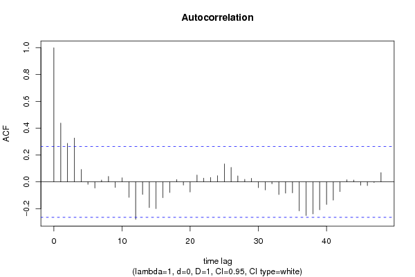
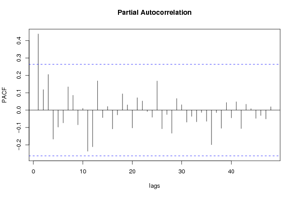
Title produced by software

(Partial) Autocorrelation Function

Date of computation

Fri, 10 Dec 2010 19:42:59 +0000

Cite this page as follows

Statistical Computations at FreeStatistics.org, Office for Research Development and Education, URL https://freestatistics.org/blog/index.php?v=date/2010/Dec/10/t1292010058t9ksmmq995exudb.htm/, Retrieved Mon, 29 Apr 2024 11:52:49 +0000

Statistical Computations at FreeStatistics.org, Office for Research Development and Education, URL https://freestatistics.org/blog/index.php?pk=107910, Retrieved Mon, 29 Apr 2024 11:52:49 +0000

QR Codes:

Paste this QR Code to cite your computation.

Original text written by user:

IsPrivate?

No (this computation is public)

User-defined keywords

Estimated Impact

126

Family? (F = Feedback message, R = changed R code, M = changed R Module, P = changed Parameters, D = changed Data)

-     [Univariate Explorative Data Analysis] [Run Sequence gebo...] [2008-12-12 13:32:37] [76963dc1903f0f612b6153510a3818cf]
- R  D  [Univariate Explorative Data Analysis] [Run Sequence gebo...] [2008-12-17 12:14:40] [76963dc1903f0f612b6153510a3818cf]
-         [Univariate Explorative Data Analysis] [Run Sequence Plot...] [2008-12-22 18:19:51] [1ce0d16c8f4225c977b42c8fa93bc163]
- RMP       [(Partial) Autocorrelation Function] [Identifying Integ...] [2009-11-22 12:16:10] [b98453cac15ba1066b407e146608df68]
- R  D        [(Partial) Autocorrelation Function] [] [2009-11-27 12:15:02] [ebd107afac1bd6180acb277edd05815b]
- R PD          [(Partial) Autocorrelation Function] [# bouwvergunninge...] [2010-12-10 19:29:44] [05ab9592748364013445d860bb938e43]
-   P               [(Partial) Autocorrelation Function] [# bouwvergunninge...] [2010-12-10 19:42:59] [60147a93d53c93401a082f47876e6cb5] [Current]

Feedback Forum

Post a new message

Dataseries X:

Download CSV

Histogram

Boxplots

Summary of computational transaction
Raw Input	view raw input (R code)
Raw Output	view raw output of R engine
Computing time	2 seconds
R Server	'Sir Ronald Aylmer Fisher' @ 193.190.124.24

\begin{tabular}{lllllllll}
\hline
Summary of computational transaction \tabularnewline
Raw Input & view raw input (R code)  \tabularnewline
Raw Output & view raw output of R engine  \tabularnewline
Computing time & 2 seconds \tabularnewline
R Server & 'Sir Ronald Aylmer Fisher' @ 193.190.124.24 \tabularnewline
\hline
\end{tabular}
%Source: https://freestatistics.org/blog/index.php?pk=107910&T=0

[TABLE]
[ROW][C]Summary of computational transaction[/C][/ROW]
[ROW][C]Raw Input[/C][C]view raw input (R code) [/C][/ROW]
[ROW][C]Raw Output[/C][C]view raw output of R engine [/C][/ROW]
[ROW][C]Computing time[/C][C]2 seconds[/C][/ROW]
[ROW][C]R Server[/C][C]'Sir Ronald Aylmer Fisher' @ 193.190.124.24[/C][/ROW]
[/TABLE]
Source: https://freestatistics.org/blog/index.php?pk=107910&T=0

Globally Unique Identifier (entire table): ba.freestatistics.org/blog/index.php?pk=107910&T=0

As an alternative you can also use a QR Code:

The GUIDs for individual cells are displayed in the table below:

Summary of computational transaction
Raw Input	view raw input (R code)
Raw Output	view raw output of R engine
Computing time	2 seconds
R Server	'Sir Ronald Aylmer Fisher' @ 193.190.124.24

Autocorrelation Function
Time lag k	ACF(k)	T-STAT	P-value
1	0.438708	3.2535	0.000976
2	0.287623	2.1331	0.018698
3	0.326532	2.4216	0.009388
4	0.091879	0.6814	0.24924
5	-0.018399	-0.1365	0.445981
6	-0.046366	-0.3439	0.366131
7	0.013222	0.0981	0.461121
8	0.040196	0.2981	0.383374
9	-0.041561	-0.3082	0.379539
10	0.030814	0.2285	0.410043
11	-0.115609	-0.8574	0.197478
12	-0.279136	-2.0701	0.021574
13	-0.094228	-0.6988	0.243806
14	-0.192016	-1.424	0.080043
15	-0.200236	-1.485	0.071628
16	-0.118588	-0.8795	0.191486
17	-0.080079	-0.5939	0.277514
18	0.017151	0.1272	0.449625
19	-0.024069	-0.1785	0.429492
20	-0.075789	-0.5621	0.288176
21	0.050972	0.378	0.353437
22	0.02761	0.2048	0.419257
23	0.033239	0.2465	0.403103
24	0.04537	0.3365	0.368897
25	0.13379	0.9922	0.16272
26	0.108161	0.8021	0.21296
27	0.044934	0.3332	0.37011
28	0.018909	0.1402	0.444496
29	0.026746	0.1984	0.421749
30	-0.043615	-0.3235	0.373787
31	-0.060523	-0.4488	0.327652
32	-0.015634	-0.1159	0.454058
33	-0.094452	-0.7005	0.243291
34	-0.084302	-0.6252	0.267212
35	-0.082292	-0.6103	0.272091
36	-0.216646	-1.6067	0.056925
37	-0.251361	-1.8641	0.033821
38	-0.239028	-1.7727	0.04091
39	-0.208809	-1.5486	0.06361
40	-0.168731	-1.2513	0.108053
41	-0.136438	-1.0119	0.158019
42	-0.072464	-0.5374	0.296576
43	0.016241	0.1204	0.452284
44	0.01363	0.1011	0.459927
45	-0.025628	-0.1901	0.424981
46	-0.027652	-0.2051	0.419138
47	-0.00445	-0.033	0.486896
48	0.06874	0.5098	0.30612

\begin{tabular}{lllllllll}
\hline
Autocorrelation Function \tabularnewline
Time lag k & ACF(k) & T-STAT & P-value \tabularnewline
1 & 0.438708 & 3.2535 & 0.000976 \tabularnewline
2 & 0.287623 & 2.1331 & 0.018698 \tabularnewline
3 & 0.326532 & 2.4216 & 0.009388 \tabularnewline
4 & 0.091879 & 0.6814 & 0.24924 \tabularnewline
5 & -0.018399 & -0.1365 & 0.445981 \tabularnewline
6 & -0.046366 & -0.3439 & 0.366131 \tabularnewline
7 & 0.013222 & 0.0981 & 0.461121 \tabularnewline
8 & 0.040196 & 0.2981 & 0.383374 \tabularnewline
9 & -0.041561 & -0.3082 & 0.379539 \tabularnewline
10 & 0.030814 & 0.2285 & 0.410043 \tabularnewline
11 & -0.115609 & -0.8574 & 0.197478 \tabularnewline
12 & -0.279136 & -2.0701 & 0.021574 \tabularnewline
13 & -0.094228 & -0.6988 & 0.243806 \tabularnewline
14 & -0.192016 & -1.424 & 0.080043 \tabularnewline
15 & -0.200236 & -1.485 & 0.071628 \tabularnewline
16 & -0.118588 & -0.8795 & 0.191486 \tabularnewline
17 & -0.080079 & -0.5939 & 0.277514 \tabularnewline
18 & 0.017151 & 0.1272 & 0.449625 \tabularnewline
19 & -0.024069 & -0.1785 & 0.429492 \tabularnewline
20 & -0.075789 & -0.5621 & 0.288176 \tabularnewline
21 & 0.050972 & 0.378 & 0.353437 \tabularnewline
22 & 0.02761 & 0.2048 & 0.419257 \tabularnewline
23 & 0.033239 & 0.2465 & 0.403103 \tabularnewline
24 & 0.04537 & 0.3365 & 0.368897 \tabularnewline
25 & 0.13379 & 0.9922 & 0.16272 \tabularnewline
26 & 0.108161 & 0.8021 & 0.21296 \tabularnewline
27 & 0.044934 & 0.3332 & 0.37011 \tabularnewline
28 & 0.018909 & 0.1402 & 0.444496 \tabularnewline
29 & 0.026746 & 0.1984 & 0.421749 \tabularnewline
30 & -0.043615 & -0.3235 & 0.373787 \tabularnewline
31 & -0.060523 & -0.4488 & 0.327652 \tabularnewline
32 & -0.015634 & -0.1159 & 0.454058 \tabularnewline
33 & -0.094452 & -0.7005 & 0.243291 \tabularnewline
34 & -0.084302 & -0.6252 & 0.267212 \tabularnewline
35 & -0.082292 & -0.6103 & 0.272091 \tabularnewline
36 & -0.216646 & -1.6067 & 0.056925 \tabularnewline
37 & -0.251361 & -1.8641 & 0.033821 \tabularnewline
38 & -0.239028 & -1.7727 & 0.04091 \tabularnewline
39 & -0.208809 & -1.5486 & 0.06361 \tabularnewline
40 & -0.168731 & -1.2513 & 0.108053 \tabularnewline
41 & -0.136438 & -1.0119 & 0.158019 \tabularnewline
42 & -0.072464 & -0.5374 & 0.296576 \tabularnewline
43 & 0.016241 & 0.1204 & 0.452284 \tabularnewline
44 & 0.01363 & 0.1011 & 0.459927 \tabularnewline
45 & -0.025628 & -0.1901 & 0.424981 \tabularnewline
46 & -0.027652 & -0.2051 & 0.419138 \tabularnewline
47 & -0.00445 & -0.033 & 0.486896 \tabularnewline
48 & 0.06874 & 0.5098 & 0.30612 \tabularnewline
\hline
\end{tabular}
%Source: https://freestatistics.org/blog/index.php?pk=107910&T=1

[TABLE]
[ROW][C]Autocorrelation Function[/C][/ROW]
[ROW][C]Time lag k[/C][C]ACF(k)[/C][C]T-STAT[/C][C]P-value[/C][/ROW]
[ROW][C]1[/C][C]0.438708[/C][C]3.2535[/C][C]0.000976[/C][/ROW]
[ROW][C]2[/C][C]0.287623[/C][C]2.1331[/C][C]0.018698[/C][/ROW]
[ROW][C]3[/C][C]0.326532[/C][C]2.4216[/C][C]0.009388[/C][/ROW]
[ROW][C]4[/C][C]0.091879[/C][C]0.6814[/C][C]0.24924[/C][/ROW]
[ROW][C]5[/C][C]-0.018399[/C][C]-0.1365[/C][C]0.445981[/C][/ROW]
[ROW][C]6[/C][C]-0.046366[/C][C]-0.3439[/C][C]0.366131[/C][/ROW]
[ROW][C]7[/C][C]0.013222[/C][C]0.0981[/C][C]0.461121[/C][/ROW]
[ROW][C]8[/C][C]0.040196[/C][C]0.2981[/C][C]0.383374[/C][/ROW]
[ROW][C]9[/C][C]-0.041561[/C][C]-0.3082[/C][C]0.379539[/C][/ROW]
[ROW][C]10[/C][C]0.030814[/C][C]0.2285[/C][C]0.410043[/C][/ROW]
[ROW][C]11[/C][C]-0.115609[/C][C]-0.8574[/C][C]0.197478[/C][/ROW]
[ROW][C]12[/C][C]-0.279136[/C][C]-2.0701[/C][C]0.021574[/C][/ROW]
[ROW][C]13[/C][C]-0.094228[/C][C]-0.6988[/C][C]0.243806[/C][/ROW]
[ROW][C]14[/C][C]-0.192016[/C][C]-1.424[/C][C]0.080043[/C][/ROW]
[ROW][C]15[/C][C]-0.200236[/C][C]-1.485[/C][C]0.071628[/C][/ROW]
[ROW][C]16[/C][C]-0.118588[/C][C]-0.8795[/C][C]0.191486[/C][/ROW]
[ROW][C]17[/C][C]-0.080079[/C][C]-0.5939[/C][C]0.277514[/C][/ROW]
[ROW][C]18[/C][C]0.017151[/C][C]0.1272[/C][C]0.449625[/C][/ROW]
[ROW][C]19[/C][C]-0.024069[/C][C]-0.1785[/C][C]0.429492[/C][/ROW]
[ROW][C]20[/C][C]-0.075789[/C][C]-0.5621[/C][C]0.288176[/C][/ROW]
[ROW][C]21[/C][C]0.050972[/C][C]0.378[/C][C]0.353437[/C][/ROW]
[ROW][C]22[/C][C]0.02761[/C][C]0.2048[/C][C]0.419257[/C][/ROW]
[ROW][C]23[/C][C]0.033239[/C][C]0.2465[/C][C]0.403103[/C][/ROW]
[ROW][C]24[/C][C]0.04537[/C][C]0.3365[/C][C]0.368897[/C][/ROW]
[ROW][C]25[/C][C]0.13379[/C][C]0.9922[/C][C]0.16272[/C][/ROW]
[ROW][C]26[/C][C]0.108161[/C][C]0.8021[/C][C]0.21296[/C][/ROW]
[ROW][C]27[/C][C]0.044934[/C][C]0.3332[/C][C]0.37011[/C][/ROW]
[ROW][C]28[/C][C]0.018909[/C][C]0.1402[/C][C]0.444496[/C][/ROW]
[ROW][C]29[/C][C]0.026746[/C][C]0.1984[/C][C]0.421749[/C][/ROW]
[ROW][C]30[/C][C]-0.043615[/C][C]-0.3235[/C][C]0.373787[/C][/ROW]
[ROW][C]31[/C][C]-0.060523[/C][C]-0.4488[/C][C]0.327652[/C][/ROW]
[ROW][C]32[/C][C]-0.015634[/C][C]-0.1159[/C][C]0.454058[/C][/ROW]
[ROW][C]33[/C][C]-0.094452[/C][C]-0.7005[/C][C]0.243291[/C][/ROW]
[ROW][C]34[/C][C]-0.084302[/C][C]-0.6252[/C][C]0.267212[/C][/ROW]
[ROW][C]35[/C][C]-0.082292[/C][C]-0.6103[/C][C]0.272091[/C][/ROW]
[ROW][C]36[/C][C]-0.216646[/C][C]-1.6067[/C][C]0.056925[/C][/ROW]
[ROW][C]37[/C][C]-0.251361[/C][C]-1.8641[/C][C]0.033821[/C][/ROW]
[ROW][C]38[/C][C]-0.239028[/C][C]-1.7727[/C][C]0.04091[/C][/ROW]
[ROW][C]39[/C][C]-0.208809[/C][C]-1.5486[/C][C]0.06361[/C][/ROW]
[ROW][C]40[/C][C]-0.168731[/C][C]-1.2513[/C][C]0.108053[/C][/ROW]
[ROW][C]41[/C][C]-0.136438[/C][C]-1.0119[/C][C]0.158019[/C][/ROW]
[ROW][C]42[/C][C]-0.072464[/C][C]-0.5374[/C][C]0.296576[/C][/ROW]
[ROW][C]43[/C][C]0.016241[/C][C]0.1204[/C][C]0.452284[/C][/ROW]
[ROW][C]44[/C][C]0.01363[/C][C]0.1011[/C][C]0.459927[/C][/ROW]
[ROW][C]45[/C][C]-0.025628[/C][C]-0.1901[/C][C]0.424981[/C][/ROW]
[ROW][C]46[/C][C]-0.027652[/C][C]-0.2051[/C][C]0.419138[/C][/ROW]
[ROW][C]47[/C][C]-0.00445[/C][C]-0.033[/C][C]0.486896[/C][/ROW]
[ROW][C]48[/C][C]0.06874[/C][C]0.5098[/C][C]0.30612[/C][/ROW]
[/TABLE]
Source: https://freestatistics.org/blog/index.php?pk=107910&T=1

Globally Unique Identifier (entire table): ba.freestatistics.org/blog/index.php?pk=107910&T=1

As an alternative you can also use a QR Code:

The GUIDs for individual cells are displayed in the table below:

Autocorrelation Function
Time lag k	ACF(k)	T-STAT	P-value
1	0.438708	3.2535	0.000976
2	0.287623	2.1331	0.018698
3	0.326532	2.4216	0.009388
4	0.091879	0.6814	0.24924
5	-0.018399	-0.1365	0.445981
6	-0.046366	-0.3439	0.366131
7	0.013222	0.0981	0.461121
8	0.040196	0.2981	0.383374
9	-0.041561	-0.3082	0.379539
10	0.030814	0.2285	0.410043
11	-0.115609	-0.8574	0.197478
12	-0.279136	-2.0701	0.021574
13	-0.094228	-0.6988	0.243806
14	-0.192016	-1.424	0.080043
15	-0.200236	-1.485	0.071628
16	-0.118588	-0.8795	0.191486
17	-0.080079	-0.5939	0.277514
18	0.017151	0.1272	0.449625
19	-0.024069	-0.1785	0.429492
20	-0.075789	-0.5621	0.288176
21	0.050972	0.378	0.353437
22	0.02761	0.2048	0.419257
23	0.033239	0.2465	0.403103
24	0.04537	0.3365	0.368897
25	0.13379	0.9922	0.16272
26	0.108161	0.8021	0.21296
27	0.044934	0.3332	0.37011
28	0.018909	0.1402	0.444496
29	0.026746	0.1984	0.421749
30	-0.043615	-0.3235	0.373787
31	-0.060523	-0.4488	0.327652
32	-0.015634	-0.1159	0.454058
33	-0.094452	-0.7005	0.243291
34	-0.084302	-0.6252	0.267212
35	-0.082292	-0.6103	0.272091
36	-0.216646	-1.6067	0.056925
37	-0.251361	-1.8641	0.033821
38	-0.239028	-1.7727	0.04091
39	-0.208809	-1.5486	0.06361
40	-0.168731	-1.2513	0.108053
41	-0.136438	-1.0119	0.158019
42	-0.072464	-0.5374	0.296576
43	0.016241	0.1204	0.452284
44	0.01363	0.1011	0.459927
45	-0.025628	-0.1901	0.424981
46	-0.027652	-0.2051	0.419138
47	-0.00445	-0.033	0.486896
48	0.06874	0.5098	0.30612

Partial Autocorrelation Function
Time lag k	PACF(k)	T-STAT	P-value
1	0.438708	3.2535	0.000976
2	0.117838	0.8739	0.192984
3	0.205346	1.5229	0.066758
4	-0.167439	-1.2418	0.109797
5	-0.097925	-0.7262	0.235389
6	-0.073896	-0.548	0.292947
7	0.133844	0.9926	0.162623
8	0.085529	0.6343	0.264257
9	-0.084775	-0.6287	0.266072
10	0.010326	0.0766	0.469618
11	-0.23701	-1.7577	0.04218
12	-0.211347	-1.5674	0.06138
13	0.168193	1.2474	0.108776
14	-0.043393	-0.3218	0.374407
15	0.020541	0.1523	0.439739
16	-0.10839	-0.8038	0.212475
17	-0.027493	-0.2039	0.419594
18	0.093475	0.6932	0.245541
19	0.030046	0.2228	0.412247
20	-0.102681	-0.7615	0.224806
21	0.070879	0.5257	0.300621
22	0.052382	0.3885	0.349581
23	-0.008164	-0.0605	0.475971
24	-0.041058	-0.3045	0.38095
25	0.167492	1.2422	0.109726
26	-0.107711	-0.7988	0.21392
27	-0.025361	-0.1881	0.425753
28	-0.133649	-0.9912	0.162973
29	0.06653	0.4934	0.311847
30	0.030584	0.2268	0.410705
31	-0.069497	-0.5154	0.304169
32	-0.036003	-0.267	0.395232
33	-0.06715	-0.498	0.310234
34	-0.013273	-0.0984	0.460972
35	-0.064757	-0.4802	0.316478
36	-0.199451	-1.4792	0.0724
37	-0.014189	-0.1052	0.45829
38	-0.104595	-0.7757	0.220624
39	0.043465	0.3223	0.374206
40	-0.044891	-0.3329	0.370231
41	0.047572	0.3528	0.362792
42	-0.106435	-0.7893	0.21665
43	0.033296	0.2469	0.40294
44	0.007855	0.0583	0.476879
45	-0.04775	-0.3541	0.362301
46	-0.031298	-0.2321	0.408655
47	-0.050779	-0.3766	0.353965
48	0.018922	0.1403	0.444455

\begin{tabular}{lllllllll}
\hline
Partial Autocorrelation Function \tabularnewline
Time lag k & PACF(k) & T-STAT & P-value \tabularnewline
1 & 0.438708 & 3.2535 & 0.000976 \tabularnewline
2 & 0.117838 & 0.8739 & 0.192984 \tabularnewline
3 & 0.205346 & 1.5229 & 0.066758 \tabularnewline
4 & -0.167439 & -1.2418 & 0.109797 \tabularnewline
5 & -0.097925 & -0.7262 & 0.235389 \tabularnewline
6 & -0.073896 & -0.548 & 0.292947 \tabularnewline
7 & 0.133844 & 0.9926 & 0.162623 \tabularnewline
8 & 0.085529 & 0.6343 & 0.264257 \tabularnewline
9 & -0.084775 & -0.6287 & 0.266072 \tabularnewline
10 & 0.010326 & 0.0766 & 0.469618 \tabularnewline
11 & -0.23701 & -1.7577 & 0.04218 \tabularnewline
12 & -0.211347 & -1.5674 & 0.06138 \tabularnewline
13 & 0.168193 & 1.2474 & 0.108776 \tabularnewline
14 & -0.043393 & -0.3218 & 0.374407 \tabularnewline
15 & 0.020541 & 0.1523 & 0.439739 \tabularnewline
16 & -0.10839 & -0.8038 & 0.212475 \tabularnewline
17 & -0.027493 & -0.2039 & 0.419594 \tabularnewline
18 & 0.093475 & 0.6932 & 0.245541 \tabularnewline
19 & 0.030046 & 0.2228 & 0.412247 \tabularnewline
20 & -0.102681 & -0.7615 & 0.224806 \tabularnewline
21 & 0.070879 & 0.5257 & 0.300621 \tabularnewline
22 & 0.052382 & 0.3885 & 0.349581 \tabularnewline
23 & -0.008164 & -0.0605 & 0.475971 \tabularnewline
24 & -0.041058 & -0.3045 & 0.38095 \tabularnewline
25 & 0.167492 & 1.2422 & 0.109726 \tabularnewline
26 & -0.107711 & -0.7988 & 0.21392 \tabularnewline
27 & -0.025361 & -0.1881 & 0.425753 \tabularnewline
28 & -0.133649 & -0.9912 & 0.162973 \tabularnewline
29 & 0.06653 & 0.4934 & 0.311847 \tabularnewline
30 & 0.030584 & 0.2268 & 0.410705 \tabularnewline
31 & -0.069497 & -0.5154 & 0.304169 \tabularnewline
32 & -0.036003 & -0.267 & 0.395232 \tabularnewline
33 & -0.06715 & -0.498 & 0.310234 \tabularnewline
34 & -0.013273 & -0.0984 & 0.460972 \tabularnewline
35 & -0.064757 & -0.4802 & 0.316478 \tabularnewline
36 & -0.199451 & -1.4792 & 0.0724 \tabularnewline
37 & -0.014189 & -0.1052 & 0.45829 \tabularnewline
38 & -0.104595 & -0.7757 & 0.220624 \tabularnewline
39 & 0.043465 & 0.3223 & 0.374206 \tabularnewline
40 & -0.044891 & -0.3329 & 0.370231 \tabularnewline
41 & 0.047572 & 0.3528 & 0.362792 \tabularnewline
42 & -0.106435 & -0.7893 & 0.21665 \tabularnewline
43 & 0.033296 & 0.2469 & 0.40294 \tabularnewline
44 & 0.007855 & 0.0583 & 0.476879 \tabularnewline
45 & -0.04775 & -0.3541 & 0.362301 \tabularnewline
46 & -0.031298 & -0.2321 & 0.408655 \tabularnewline
47 & -0.050779 & -0.3766 & 0.353965 \tabularnewline
48 & 0.018922 & 0.1403 & 0.444455 \tabularnewline
\hline
\end{tabular}
%Source: https://freestatistics.org/blog/index.php?pk=107910&T=2

[TABLE]
[ROW][C]Partial Autocorrelation Function[/C][/ROW]
[ROW][C]Time lag k[/C][C]PACF(k)[/C][C]T-STAT[/C][C]P-value[/C][/ROW]
[ROW][C]1[/C][C]0.438708[/C][C]3.2535[/C][C]0.000976[/C][/ROW]
[ROW][C]2[/C][C]0.117838[/C][C]0.8739[/C][C]0.192984[/C][/ROW]
[ROW][C]3[/C][C]0.205346[/C][C]1.5229[/C][C]0.066758[/C][/ROW]
[ROW][C]4[/C][C]-0.167439[/C][C]-1.2418[/C][C]0.109797[/C][/ROW]
[ROW][C]5[/C][C]-0.097925[/C][C]-0.7262[/C][C]0.235389[/C][/ROW]
[ROW][C]6[/C][C]-0.073896[/C][C]-0.548[/C][C]0.292947[/C][/ROW]
[ROW][C]7[/C][C]0.133844[/C][C]0.9926[/C][C]0.162623[/C][/ROW]
[ROW][C]8[/C][C]0.085529[/C][C]0.6343[/C][C]0.264257[/C][/ROW]
[ROW][C]9[/C][C]-0.084775[/C][C]-0.6287[/C][C]0.266072[/C][/ROW]
[ROW][C]10[/C][C]0.010326[/C][C]0.0766[/C][C]0.469618[/C][/ROW]
[ROW][C]11[/C][C]-0.23701[/C][C]-1.7577[/C][C]0.04218[/C][/ROW]
[ROW][C]12[/C][C]-0.211347[/C][C]-1.5674[/C][C]0.06138[/C][/ROW]
[ROW][C]13[/C][C]0.168193[/C][C]1.2474[/C][C]0.108776[/C][/ROW]
[ROW][C]14[/C][C]-0.043393[/C][C]-0.3218[/C][C]0.374407[/C][/ROW]
[ROW][C]15[/C][C]0.020541[/C][C]0.1523[/C][C]0.439739[/C][/ROW]
[ROW][C]16[/C][C]-0.10839[/C][C]-0.8038[/C][C]0.212475[/C][/ROW]
[ROW][C]17[/C][C]-0.027493[/C][C]-0.2039[/C][C]0.419594[/C][/ROW]
[ROW][C]18[/C][C]0.093475[/C][C]0.6932[/C][C]0.245541[/C][/ROW]
[ROW][C]19[/C][C]0.030046[/C][C]0.2228[/C][C]0.412247[/C][/ROW]
[ROW][C]20[/C][C]-0.102681[/C][C]-0.7615[/C][C]0.224806[/C][/ROW]
[ROW][C]21[/C][C]0.070879[/C][C]0.5257[/C][C]0.300621[/C][/ROW]
[ROW][C]22[/C][C]0.052382[/C][C]0.3885[/C][C]0.349581[/C][/ROW]
[ROW][C]23[/C][C]-0.008164[/C][C]-0.0605[/C][C]0.475971[/C][/ROW]
[ROW][C]24[/C][C]-0.041058[/C][C]-0.3045[/C][C]0.38095[/C][/ROW]
[ROW][C]25[/C][C]0.167492[/C][C]1.2422[/C][C]0.109726[/C][/ROW]
[ROW][C]26[/C][C]-0.107711[/C][C]-0.7988[/C][C]0.21392[/C][/ROW]
[ROW][C]27[/C][C]-0.025361[/C][C]-0.1881[/C][C]0.425753[/C][/ROW]
[ROW][C]28[/C][C]-0.133649[/C][C]-0.9912[/C][C]0.162973[/C][/ROW]
[ROW][C]29[/C][C]0.06653[/C][C]0.4934[/C][C]0.311847[/C][/ROW]
[ROW][C]30[/C][C]0.030584[/C][C]0.2268[/C][C]0.410705[/C][/ROW]
[ROW][C]31[/C][C]-0.069497[/C][C]-0.5154[/C][C]0.304169[/C][/ROW]
[ROW][C]32[/C][C]-0.036003[/C][C]-0.267[/C][C]0.395232[/C][/ROW]
[ROW][C]33[/C][C]-0.06715[/C][C]-0.498[/C][C]0.310234[/C][/ROW]
[ROW][C]34[/C][C]-0.013273[/C][C]-0.0984[/C][C]0.460972[/C][/ROW]
[ROW][C]35[/C][C]-0.064757[/C][C]-0.4802[/C][C]0.316478[/C][/ROW]
[ROW][C]36[/C][C]-0.199451[/C][C]-1.4792[/C][C]0.0724[/C][/ROW]
[ROW][C]37[/C][C]-0.014189[/C][C]-0.1052[/C][C]0.45829[/C][/ROW]
[ROW][C]38[/C][C]-0.104595[/C][C]-0.7757[/C][C]0.220624[/C][/ROW]
[ROW][C]39[/C][C]0.043465[/C][C]0.3223[/C][C]0.374206[/C][/ROW]
[ROW][C]40[/C][C]-0.044891[/C][C]-0.3329[/C][C]0.370231[/C][/ROW]
[ROW][C]41[/C][C]0.047572[/C][C]0.3528[/C][C]0.362792[/C][/ROW]
[ROW][C]42[/C][C]-0.106435[/C][C]-0.7893[/C][C]0.21665[/C][/ROW]
[ROW][C]43[/C][C]0.033296[/C][C]0.2469[/C][C]0.40294[/C][/ROW]
[ROW][C]44[/C][C]0.007855[/C][C]0.0583[/C][C]0.476879[/C][/ROW]
[ROW][C]45[/C][C]-0.04775[/C][C]-0.3541[/C][C]0.362301[/C][/ROW]
[ROW][C]46[/C][C]-0.031298[/C][C]-0.2321[/C][C]0.408655[/C][/ROW]
[ROW][C]47[/C][C]-0.050779[/C][C]-0.3766[/C][C]0.353965[/C][/ROW]
[ROW][C]48[/C][C]0.018922[/C][C]0.1403[/C][C]0.444455[/C][/ROW]
[/TABLE]
Source: https://freestatistics.org/blog/index.php?pk=107910&T=2

Globally Unique Identifier (entire table): ba.freestatistics.org/blog/index.php?pk=107910&T=2

As an alternative you can also use a QR Code:

The GUIDs for individual cells are displayed in the table below:

Partial Autocorrelation Function
Time lag k	PACF(k)	T-STAT	P-value
1	0.438708	3.2535	0.000976
2	0.117838	0.8739	0.192984
3	0.205346	1.5229	0.066758
4	-0.167439	-1.2418	0.109797
5	-0.097925	-0.7262	0.235389
6	-0.073896	-0.548	0.292947
7	0.133844	0.9926	0.162623
8	0.085529	0.6343	0.264257
9	-0.084775	-0.6287	0.266072
10	0.010326	0.0766	0.469618
11	-0.23701	-1.7577	0.04218
12	-0.211347	-1.5674	0.06138
13	0.168193	1.2474	0.108776
14	-0.043393	-0.3218	0.374407
15	0.020541	0.1523	0.439739
16	-0.10839	-0.8038	0.212475
17	-0.027493	-0.2039	0.419594
18	0.093475	0.6932	0.245541
19	0.030046	0.2228	0.412247
20	-0.102681	-0.7615	0.224806
21	0.070879	0.5257	0.300621
22	0.052382	0.3885	0.349581
23	-0.008164	-0.0605	0.475971
24	-0.041058	-0.3045	0.38095
25	0.167492	1.2422	0.109726
26	-0.107711	-0.7988	0.21392
27	-0.025361	-0.1881	0.425753
28	-0.133649	-0.9912	0.162973
29	0.06653	0.4934	0.311847
30	0.030584	0.2268	0.410705
31	-0.069497	-0.5154	0.304169
32	-0.036003	-0.267	0.395232
33	-0.06715	-0.498	0.310234
34	-0.013273	-0.0984	0.460972
35	-0.064757	-0.4802	0.316478
36	-0.199451	-1.4792	0.0724
37	-0.014189	-0.1052	0.45829
38	-0.104595	-0.7757	0.220624
39	0.043465	0.3223	0.374206
40	-0.044891	-0.3329	0.370231
41	0.047572	0.3528	0.362792
42	-0.106435	-0.7893	0.21665
43	0.033296	0.2469	0.40294
44	0.007855	0.0583	0.476879
45	-0.04775	-0.3541	0.362301
46	-0.031298	-0.2321	0.408655
47	-0.050779	-0.3766	0.353965
48	0.018922	0.1403	0.444455

Figure 1

PNG link

Postscript link

PDF link

Figure 2

PNG link

Postscript link

PDF link

Parameters (Session):

par1 = 48 ; par2 = 1 ; par3 = 0 ; par4 = 1 ; par5 = 12 ; par6 = White Noise ; par7 = 0.95 ;

Parameters (R input):

par1 = 48 ; par2 = 1 ; par3 = 0 ; par4 = 1 ; par5 = 12 ; par6 = White Noise ; par7 = 0.95 ;

R code (references can be found in the software module):

if (par1 == 'Default') {
par1 = 10*log10(length(x))
} else {
par1 <- as.numeric(par1)
}
par2 <- as.numeric(par2)
par3 <- as.numeric(par3)
par4 <- as.numeric(par4)
par5 <- as.numeric(par5)
if (par6 == 'White Noise') par6 <- 'white' else par6 <- 'ma'
par7 <- as.numeric(par7)
if (par2 == 0) {
x <- log(x)
} else {
x <- (x ^ par2 - 1) / par2
}
if (par3 > 0) x <- diff(x,lag=1,difference=par3)
if (par4 > 0) x <- diff(x,lag=par5,difference=par4)
bitmap(file='pic1.png')
racf <- acf(x, par1, main='Autocorrelation', xlab='time lag', ylab='ACF', ci.type=par6, ci=par7, sub=paste('(lambda=',par2,', d=',par3,', D=',par4,', CI=', par7, ', CI type=',par6,')',sep=''))
dev.off()
bitmap(file='pic2.png')
rpacf <- pacf(x,par1,main='Partial Autocorrelation',xlab='lags',ylab='PACF')
dev.off()
(myacf <- c(racf$acf))
(mypacf <- c(rpacf$acf))
lengthx <- length(x)
sqrtn <- sqrt(lengthx)
load(file='createtable')
a<-table.start()
a<-table.row.start(a)
a<-table.element(a,'Autocorrelation Function',4,TRUE)
a<-table.row.end(a)
a<-table.row.start(a)
a<-table.element(a,'Time lag k',header=TRUE)
a<-table.element(a,hyperlink('basics.htm','ACF(k)','click here for more information about the Autocorrelation Function'),header=TRUE)
a<-table.element(a,'T-STAT',header=TRUE)
a<-table.element(a,'P-value',header=TRUE)
a<-table.row.end(a)
for (i in 2:(par1+1)) {
a<-table.row.start(a)
a<-table.element(a,i-1,header=TRUE)
a<-table.element(a,round(myacf[i],6))
mytstat <- myacf[i]*sqrtn
a<-table.element(a,round(mytstat,4))
a<-table.element(a,round(1-pt(abs(mytstat),lengthx),6))
a<-table.row.end(a)
}
a<-table.end(a)
table.save(a,file='mytable.tab')
a<-table.start()
a<-table.row.start(a)
a<-table.element(a,'Partial Autocorrelation Function',4,TRUE)
a<-table.row.end(a)
a<-table.row.start(a)
a<-table.element(a,'Time lag k',header=TRUE)
a<-table.element(a,hyperlink('basics.htm','PACF(k)','click here for more information about the Partial Autocorrelation Function'),header=TRUE)
a<-table.element(a,'T-STAT',header=TRUE)
a<-table.element(a,'P-value',header=TRUE)
a<-table.row.end(a)
for (i in 1:par1) {
a<-table.row.start(a)
a<-table.element(a,i,header=TRUE)
a<-table.element(a,round(mypacf[i],6))
mytstat <- mypacf[i]*sqrtn
a<-table.element(a,round(mytstat,4))
a<-table.element(a,round(1-pt(abs(mytstat),lengthx),6))
a<-table.row.end(a)
}
a<-table.end(a)
table.save(a,file='mytable1.tab')

Free Statistics

Description of Statistical Computation

Tree of Dependent Computations

Dataset

Tables (Output of Computation)

Figures (Output of Computation)

Input Parameters & R Code