Repository of Reproducible Computations

Free Statistics

of Irreproducible Research!

Author's title

Author

*The author of this computation has been verified*

R Software Module

rwasp_autocorrelation.wasp

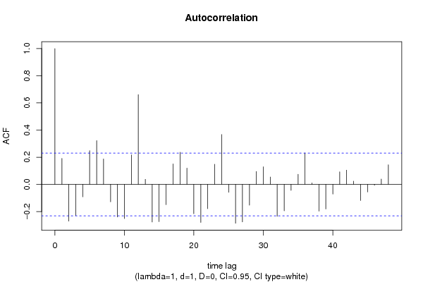
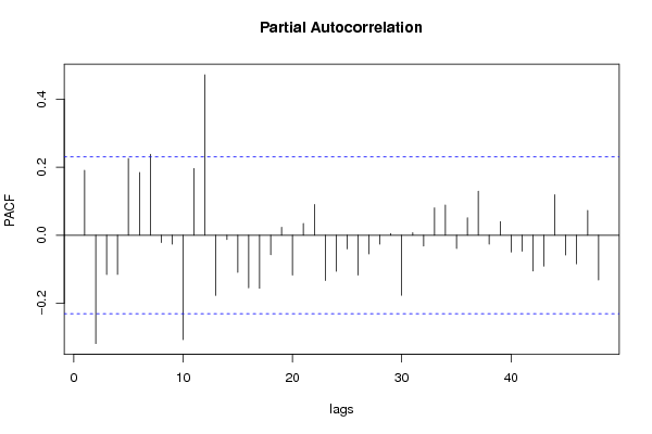
Title produced by software

(Partial) Autocorrelation Function

Date of computation

Fri, 10 Dec 2010 18:54:39 +0000

Cite this page as follows

Statistical Computations at FreeStatistics.org, Office for Research Development and Education, URL https://freestatistics.org/blog/index.php?v=date/2010/Dec/10/t1292007152fm4h8yxj04qvnxk.htm/, Retrieved Mon, 29 Apr 2024 16:36:24 +0000

Statistical Computations at FreeStatistics.org, Office for Research Development and Education, URL https://freestatistics.org/blog/index.php?pk=107886, Retrieved Mon, 29 Apr 2024 16:36:24 +0000

QR Codes:

Paste this QR Code to cite your computation.

Original text written by user:

IsPrivate?

No (this computation is public)

User-defined keywords

Estimated Impact

137

Family? (F = Feedback message, R = changed R code, M = changed R Module, P = changed Parameters, D = changed Data)

-     [Univariate Data Series] [data set] [2008-12-01 19:54:57] [b98453cac15ba1066b407e146608df68]
- RMP   [(Partial) Autocorrelation Function] [Unemployment] [2010-11-29 09:05:21] [b98453cac15ba1066b407e146608df68]
-    D    [(Partial) Autocorrelation Function] [Autocorrelation WS9] [2010-12-06 11:15:00] [f4dc4aa51d65be851b8508203d9f6001]
- R  D      [(Partial) Autocorrelation Function] [] [2010-12-06 16:49:38] [d39e5c40c631ed6c22677d2e41dbfc7d]
-   P         [(Partial) Autocorrelation Function] [Blog 1] [2010-12-10 11:09:03] [1aa8d85d6b335d32b1f6be940e33a166]
-   PD            [(Partial) Autocorrelation Function] [Verbetering student] [2010-12-10 18:54:39] [47bfda5353cd53c1cf7ea7aa9038654a] [Current]

Feedback Forum

Post a new message

Dataseries X:

Download CSV

Histogram

Boxplots

Summary of computational transaction
Raw Input	view raw input (R code)
Raw Output	view raw output of R engine
Computing time	2 seconds
R Server	'RServer@AstonUniversity' @ vre.aston.ac.uk

\begin{tabular}{lllllllll}
\hline
Summary of computational transaction \tabularnewline
Raw Input & view raw input (R code)  \tabularnewline
Raw Output & view raw output of R engine  \tabularnewline
Computing time & 2 seconds \tabularnewline
R Server & 'RServer@AstonUniversity' @ vre.aston.ac.uk \tabularnewline
\hline
\end{tabular}
%Source: https://freestatistics.org/blog/index.php?pk=107886&T=0

[TABLE]
[ROW][C]Summary of computational transaction[/C][/ROW]
[ROW][C]Raw Input[/C][C]view raw input (R code) [/C][/ROW]
[ROW][C]Raw Output[/C][C]view raw output of R engine [/C][/ROW]
[ROW][C]Computing time[/C][C]2 seconds[/C][/ROW]
[ROW][C]R Server[/C][C]'RServer@AstonUniversity' @ vre.aston.ac.uk[/C][/ROW]
[/TABLE]
Source: https://freestatistics.org/blog/index.php?pk=107886&T=0

Globally Unique Identifier (entire table): ba.freestatistics.org/blog/index.php?pk=107886&T=0

As an alternative you can also use a QR Code:

The GUIDs for individual cells are displayed in the table below:

Summary of computational transaction
Raw Input	view raw input (R code)
Raw Output	view raw output of R engine
Computing time	2 seconds
R Server	'RServer@AstonUniversity' @ vre.aston.ac.uk

Autocorrelation Function
Time lag k	ACF(k)	T-STAT	P-value
1	0.191177	1.6222	0.054567
2	-0.270518	-2.2954	0.012312
3	-0.229046	-1.9435	0.027931
4	-0.091405	-0.7756	0.220264
5	0.248245	2.1064	0.019326
6	0.32263	2.7376	0.003896
7	0.187219	1.5886	0.058266
8	-0.12869	-1.092	0.139243
9	-0.240091	-2.0372	0.022651
10	-0.251644	-2.1353	0.018071
11	0.216986	1.8412	0.034857
12	0.661234	5.6108	0
13	0.037445	0.3177	0.375804
14	-0.277019	-2.3506	0.010743
15	-0.274547	-2.3296	0.011318
16	-0.149717	-1.2704	0.104018
17	0.150552	1.2775	0.10277
18	0.23642	2.0061	0.024302
19	0.119859	1.017	0.156271
20	-0.216157	-1.8342	0.035381
21	-0.280022	-2.3761	0.010081
22	-0.17915	-1.5201	0.066428
23	0.148448	1.2596	0.105937
24	0.3671	3.115	0.001321
25	-0.057972	-0.4919	0.31214
26	-0.286203	-2.4285	0.00883
27	-0.276869	-2.3493	0.010777
28	-0.153118	-1.2993	0.099001
29	0.095564	0.8109	0.210051
30	0.129453	1.0984	0.137835
31	0.054066	0.4588	0.323893
32	-0.23493	-1.9934	0.025001
33	-0.194458	-1.65	0.051647
34	-0.043707	-0.3709	0.355913
35	0.074556	0.6326	0.264491
36	0.231692	1.966	0.026579
37	0.010971	0.0931	0.463045
38	-0.19691	-1.6708	0.049548
39	-0.181001	-1.5358	0.06448
40	-0.071615	-0.6077	0.272659
41	0.092712	0.7867	0.217024
42	0.104877	0.8899	0.18824
43	0.024023	0.2038	0.419525
44	-0.118849	-1.0085	0.158303
45	-0.055413	-0.4702	0.319817
46	-0.006329	-0.0537	0.47866
47	0.038991	0.3308	0.370861
48	0.144451	1.2257	0.112152

\begin{tabular}{lllllllll}
\hline
Autocorrelation Function \tabularnewline
Time lag k & ACF(k) & T-STAT & P-value \tabularnewline
1 & 0.191177 & 1.6222 & 0.054567 \tabularnewline
2 & -0.270518 & -2.2954 & 0.012312 \tabularnewline
3 & -0.229046 & -1.9435 & 0.027931 \tabularnewline
4 & -0.091405 & -0.7756 & 0.220264 \tabularnewline
5 & 0.248245 & 2.1064 & 0.019326 \tabularnewline
6 & 0.32263 & 2.7376 & 0.003896 \tabularnewline
7 & 0.187219 & 1.5886 & 0.058266 \tabularnewline
8 & -0.12869 & -1.092 & 0.139243 \tabularnewline
9 & -0.240091 & -2.0372 & 0.022651 \tabularnewline
10 & -0.251644 & -2.1353 & 0.018071 \tabularnewline
11 & 0.216986 & 1.8412 & 0.034857 \tabularnewline
12 & 0.661234 & 5.6108 & 0 \tabularnewline
13 & 0.037445 & 0.3177 & 0.375804 \tabularnewline
14 & -0.277019 & -2.3506 & 0.010743 \tabularnewline
15 & -0.274547 & -2.3296 & 0.011318 \tabularnewline
16 & -0.149717 & -1.2704 & 0.104018 \tabularnewline
17 & 0.150552 & 1.2775 & 0.10277 \tabularnewline
18 & 0.23642 & 2.0061 & 0.024302 \tabularnewline
19 & 0.119859 & 1.017 & 0.156271 \tabularnewline
20 & -0.216157 & -1.8342 & 0.035381 \tabularnewline
21 & -0.280022 & -2.3761 & 0.010081 \tabularnewline
22 & -0.17915 & -1.5201 & 0.066428 \tabularnewline
23 & 0.148448 & 1.2596 & 0.105937 \tabularnewline
24 & 0.3671 & 3.115 & 0.001321 \tabularnewline
25 & -0.057972 & -0.4919 & 0.31214 \tabularnewline
26 & -0.286203 & -2.4285 & 0.00883 \tabularnewline
27 & -0.276869 & -2.3493 & 0.010777 \tabularnewline
28 & -0.153118 & -1.2993 & 0.099001 \tabularnewline
29 & 0.095564 & 0.8109 & 0.210051 \tabularnewline
30 & 0.129453 & 1.0984 & 0.137835 \tabularnewline
31 & 0.054066 & 0.4588 & 0.323893 \tabularnewline
32 & -0.23493 & -1.9934 & 0.025001 \tabularnewline
33 & -0.194458 & -1.65 & 0.051647 \tabularnewline
34 & -0.043707 & -0.3709 & 0.355913 \tabularnewline
35 & 0.074556 & 0.6326 & 0.264491 \tabularnewline
36 & 0.231692 & 1.966 & 0.026579 \tabularnewline
37 & 0.010971 & 0.0931 & 0.463045 \tabularnewline
38 & -0.19691 & -1.6708 & 0.049548 \tabularnewline
39 & -0.181001 & -1.5358 & 0.06448 \tabularnewline
40 & -0.071615 & -0.6077 & 0.272659 \tabularnewline
41 & 0.092712 & 0.7867 & 0.217024 \tabularnewline
42 & 0.104877 & 0.8899 & 0.18824 \tabularnewline
43 & 0.024023 & 0.2038 & 0.419525 \tabularnewline
44 & -0.118849 & -1.0085 & 0.158303 \tabularnewline
45 & -0.055413 & -0.4702 & 0.319817 \tabularnewline
46 & -0.006329 & -0.0537 & 0.47866 \tabularnewline
47 & 0.038991 & 0.3308 & 0.370861 \tabularnewline
48 & 0.144451 & 1.2257 & 0.112152 \tabularnewline
\hline
\end{tabular}
%Source: https://freestatistics.org/blog/index.php?pk=107886&T=1

[TABLE]
[ROW][C]Autocorrelation Function[/C][/ROW]
[ROW][C]Time lag k[/C][C]ACF(k)[/C][C]T-STAT[/C][C]P-value[/C][/ROW]
[ROW][C]1[/C][C]0.191177[/C][C]1.6222[/C][C]0.054567[/C][/ROW]
[ROW][C]2[/C][C]-0.270518[/C][C]-2.2954[/C][C]0.012312[/C][/ROW]
[ROW][C]3[/C][C]-0.229046[/C][C]-1.9435[/C][C]0.027931[/C][/ROW]
[ROW][C]4[/C][C]-0.091405[/C][C]-0.7756[/C][C]0.220264[/C][/ROW]
[ROW][C]5[/C][C]0.248245[/C][C]2.1064[/C][C]0.019326[/C][/ROW]
[ROW][C]6[/C][C]0.32263[/C][C]2.7376[/C][C]0.003896[/C][/ROW]
[ROW][C]7[/C][C]0.187219[/C][C]1.5886[/C][C]0.058266[/C][/ROW]
[ROW][C]8[/C][C]-0.12869[/C][C]-1.092[/C][C]0.139243[/C][/ROW]
[ROW][C]9[/C][C]-0.240091[/C][C]-2.0372[/C][C]0.022651[/C][/ROW]
[ROW][C]10[/C][C]-0.251644[/C][C]-2.1353[/C][C]0.018071[/C][/ROW]
[ROW][C]11[/C][C]0.216986[/C][C]1.8412[/C][C]0.034857[/C][/ROW]
[ROW][C]12[/C][C]0.661234[/C][C]5.6108[/C][C]0[/C][/ROW]
[ROW][C]13[/C][C]0.037445[/C][C]0.3177[/C][C]0.375804[/C][/ROW]
[ROW][C]14[/C][C]-0.277019[/C][C]-2.3506[/C][C]0.010743[/C][/ROW]
[ROW][C]15[/C][C]-0.274547[/C][C]-2.3296[/C][C]0.011318[/C][/ROW]
[ROW][C]16[/C][C]-0.149717[/C][C]-1.2704[/C][C]0.104018[/C][/ROW]
[ROW][C]17[/C][C]0.150552[/C][C]1.2775[/C][C]0.10277[/C][/ROW]
[ROW][C]18[/C][C]0.23642[/C][C]2.0061[/C][C]0.024302[/C][/ROW]
[ROW][C]19[/C][C]0.119859[/C][C]1.017[/C][C]0.156271[/C][/ROW]
[ROW][C]20[/C][C]-0.216157[/C][C]-1.8342[/C][C]0.035381[/C][/ROW]
[ROW][C]21[/C][C]-0.280022[/C][C]-2.3761[/C][C]0.010081[/C][/ROW]
[ROW][C]22[/C][C]-0.17915[/C][C]-1.5201[/C][C]0.066428[/C][/ROW]
[ROW][C]23[/C][C]0.148448[/C][C]1.2596[/C][C]0.105937[/C][/ROW]
[ROW][C]24[/C][C]0.3671[/C][C]3.115[/C][C]0.001321[/C][/ROW]
[ROW][C]25[/C][C]-0.057972[/C][C]-0.4919[/C][C]0.31214[/C][/ROW]
[ROW][C]26[/C][C]-0.286203[/C][C]-2.4285[/C][C]0.00883[/C][/ROW]
[ROW][C]27[/C][C]-0.276869[/C][C]-2.3493[/C][C]0.010777[/C][/ROW]
[ROW][C]28[/C][C]-0.153118[/C][C]-1.2993[/C][C]0.099001[/C][/ROW]
[ROW][C]29[/C][C]0.095564[/C][C]0.8109[/C][C]0.210051[/C][/ROW]
[ROW][C]30[/C][C]0.129453[/C][C]1.0984[/C][C]0.137835[/C][/ROW]
[ROW][C]31[/C][C]0.054066[/C][C]0.4588[/C][C]0.323893[/C][/ROW]
[ROW][C]32[/C][C]-0.23493[/C][C]-1.9934[/C][C]0.025001[/C][/ROW]
[ROW][C]33[/C][C]-0.194458[/C][C]-1.65[/C][C]0.051647[/C][/ROW]
[ROW][C]34[/C][C]-0.043707[/C][C]-0.3709[/C][C]0.355913[/C][/ROW]
[ROW][C]35[/C][C]0.074556[/C][C]0.6326[/C][C]0.264491[/C][/ROW]
[ROW][C]36[/C][C]0.231692[/C][C]1.966[/C][C]0.026579[/C][/ROW]
[ROW][C]37[/C][C]0.010971[/C][C]0.0931[/C][C]0.463045[/C][/ROW]
[ROW][C]38[/C][C]-0.19691[/C][C]-1.6708[/C][C]0.049548[/C][/ROW]
[ROW][C]39[/C][C]-0.181001[/C][C]-1.5358[/C][C]0.06448[/C][/ROW]
[ROW][C]40[/C][C]-0.071615[/C][C]-0.6077[/C][C]0.272659[/C][/ROW]
[ROW][C]41[/C][C]0.092712[/C][C]0.7867[/C][C]0.217024[/C][/ROW]
[ROW][C]42[/C][C]0.104877[/C][C]0.8899[/C][C]0.18824[/C][/ROW]
[ROW][C]43[/C][C]0.024023[/C][C]0.2038[/C][C]0.419525[/C][/ROW]
[ROW][C]44[/C][C]-0.118849[/C][C]-1.0085[/C][C]0.158303[/C][/ROW]
[ROW][C]45[/C][C]-0.055413[/C][C]-0.4702[/C][C]0.319817[/C][/ROW]
[ROW][C]46[/C][C]-0.006329[/C][C]-0.0537[/C][C]0.47866[/C][/ROW]
[ROW][C]47[/C][C]0.038991[/C][C]0.3308[/C][C]0.370861[/C][/ROW]
[ROW][C]48[/C][C]0.144451[/C][C]1.2257[/C][C]0.112152[/C][/ROW]
[/TABLE]
Source: https://freestatistics.org/blog/index.php?pk=107886&T=1

Globally Unique Identifier (entire table): ba.freestatistics.org/blog/index.php?pk=107886&T=1

As an alternative you can also use a QR Code:

The GUIDs for individual cells are displayed in the table below:

Autocorrelation Function
Time lag k	ACF(k)	T-STAT	P-value
1	0.191177	1.6222	0.054567
2	-0.270518	-2.2954	0.012312
3	-0.229046	-1.9435	0.027931
4	-0.091405	-0.7756	0.220264
5	0.248245	2.1064	0.019326
6	0.32263	2.7376	0.003896
7	0.187219	1.5886	0.058266
8	-0.12869	-1.092	0.139243
9	-0.240091	-2.0372	0.022651
10	-0.251644	-2.1353	0.018071
11	0.216986	1.8412	0.034857
12	0.661234	5.6108	0
13	0.037445	0.3177	0.375804
14	-0.277019	-2.3506	0.010743
15	-0.274547	-2.3296	0.011318
16	-0.149717	-1.2704	0.104018
17	0.150552	1.2775	0.10277
18	0.23642	2.0061	0.024302
19	0.119859	1.017	0.156271
20	-0.216157	-1.8342	0.035381
21	-0.280022	-2.3761	0.010081
22	-0.17915	-1.5201	0.066428
23	0.148448	1.2596	0.105937
24	0.3671	3.115	0.001321
25	-0.057972	-0.4919	0.31214
26	-0.286203	-2.4285	0.00883
27	-0.276869	-2.3493	0.010777
28	-0.153118	-1.2993	0.099001
29	0.095564	0.8109	0.210051
30	0.129453	1.0984	0.137835
31	0.054066	0.4588	0.323893
32	-0.23493	-1.9934	0.025001
33	-0.194458	-1.65	0.051647
34	-0.043707	-0.3709	0.355913
35	0.074556	0.6326	0.264491
36	0.231692	1.966	0.026579
37	0.010971	0.0931	0.463045
38	-0.19691	-1.6708	0.049548
39	-0.181001	-1.5358	0.06448
40	-0.071615	-0.6077	0.272659
41	0.092712	0.7867	0.217024
42	0.104877	0.8899	0.18824
43	0.024023	0.2038	0.419525
44	-0.118849	-1.0085	0.158303
45	-0.055413	-0.4702	0.319817
46	-0.006329	-0.0537	0.47866
47	0.038991	0.3308	0.370861
48	0.144451	1.2257	0.112152

Partial Autocorrelation Function
Time lag k	PACF(k)	T-STAT	P-value
1	0.191177	1.6222	0.054567
2	-0.318715	-2.7044	0.004267
3	-0.115431	-0.9795	0.165315
4	-0.115174	-0.9773	0.16585
5	0.225742	1.9155	0.029701
6	0.18463	1.5666	0.060792
7	0.237993	2.0194	0.023582
8	-0.021588	-0.1832	0.427586
9	-0.02629	-0.2231	0.412053
10	-0.306992	-2.6049	0.005579
11	0.196321	1.6658	0.050046
12	0.472037	4.0054	7.4e-05
13	-0.176946	-1.5014	0.068808
14	-0.012538	-0.1064	0.457785
15	-0.109129	-0.926	0.178773
16	-0.154769	-1.3133	0.096633
17	-0.155944	-1.3232	0.094973
18	-0.057508	-0.488	0.313527
19	0.023159	0.1965	0.422381
20	-0.117431	-0.9964	0.161187
21	0.03451	0.2928	0.385248
22	0.090774	0.7702	0.221838
23	-0.133274	-1.1309	0.130932
24	-0.106121	-0.9005	0.185437
25	-0.040153	-0.3407	0.367156
26	-0.117404	-0.9962	0.161243
27	-0.054986	-0.4666	0.321108
28	-0.02634	-0.2235	0.411888
29	0.005132	0.0435	0.482692
30	-0.176714	-1.4995	0.069063
31	0.00778	0.066	0.473773
32	-0.031788	-0.2697	0.394069
33	0.080495	0.683	0.248392
34	0.088608	0.7519	0.227292
35	-0.039208	-0.3327	0.370167
36	0.051532	0.4373	0.331615
37	0.12959	1.0996	0.137584
38	-0.026525	-0.2251	0.411281
39	0.040387	0.3427	0.366412
40	-0.049251	-0.4179	0.33863
41	-0.046914	-0.3981	0.345875
42	-0.105105	-0.8918	0.187723
43	-0.090726	-0.7698	0.221957
44	0.119278	1.0121	0.157438
45	-0.058011	-0.4922	0.312025
46	-0.084089	-0.7135	0.238915
47	0.073061	0.6199	0.268627
48	-0.131756	-1.118	0.133645

\begin{tabular}{lllllllll}
\hline
Partial Autocorrelation Function \tabularnewline
Time lag k & PACF(k) & T-STAT & P-value \tabularnewline
1 & 0.191177 & 1.6222 & 0.054567 \tabularnewline
2 & -0.318715 & -2.7044 & 0.004267 \tabularnewline
3 & -0.115431 & -0.9795 & 0.165315 \tabularnewline
4 & -0.115174 & -0.9773 & 0.16585 \tabularnewline
5 & 0.225742 & 1.9155 & 0.029701 \tabularnewline
6 & 0.18463 & 1.5666 & 0.060792 \tabularnewline
7 & 0.237993 & 2.0194 & 0.023582 \tabularnewline
8 & -0.021588 & -0.1832 & 0.427586 \tabularnewline
9 & -0.02629 & -0.2231 & 0.412053 \tabularnewline
10 & -0.306992 & -2.6049 & 0.005579 \tabularnewline
11 & 0.196321 & 1.6658 & 0.050046 \tabularnewline
12 & 0.472037 & 4.0054 & 7.4e-05 \tabularnewline
13 & -0.176946 & -1.5014 & 0.068808 \tabularnewline
14 & -0.012538 & -0.1064 & 0.457785 \tabularnewline
15 & -0.109129 & -0.926 & 0.178773 \tabularnewline
16 & -0.154769 & -1.3133 & 0.096633 \tabularnewline
17 & -0.155944 & -1.3232 & 0.094973 \tabularnewline
18 & -0.057508 & -0.488 & 0.313527 \tabularnewline
19 & 0.023159 & 0.1965 & 0.422381 \tabularnewline
20 & -0.117431 & -0.9964 & 0.161187 \tabularnewline
21 & 0.03451 & 0.2928 & 0.385248 \tabularnewline
22 & 0.090774 & 0.7702 & 0.221838 \tabularnewline
23 & -0.133274 & -1.1309 & 0.130932 \tabularnewline
24 & -0.106121 & -0.9005 & 0.185437 \tabularnewline
25 & -0.040153 & -0.3407 & 0.367156 \tabularnewline
26 & -0.117404 & -0.9962 & 0.161243 \tabularnewline
27 & -0.054986 & -0.4666 & 0.321108 \tabularnewline
28 & -0.02634 & -0.2235 & 0.411888 \tabularnewline
29 & 0.005132 & 0.0435 & 0.482692 \tabularnewline
30 & -0.176714 & -1.4995 & 0.069063 \tabularnewline
31 & 0.00778 & 0.066 & 0.473773 \tabularnewline
32 & -0.031788 & -0.2697 & 0.394069 \tabularnewline
33 & 0.080495 & 0.683 & 0.248392 \tabularnewline
34 & 0.088608 & 0.7519 & 0.227292 \tabularnewline
35 & -0.039208 & -0.3327 & 0.370167 \tabularnewline
36 & 0.051532 & 0.4373 & 0.331615 \tabularnewline
37 & 0.12959 & 1.0996 & 0.137584 \tabularnewline
38 & -0.026525 & -0.2251 & 0.411281 \tabularnewline
39 & 0.040387 & 0.3427 & 0.366412 \tabularnewline
40 & -0.049251 & -0.4179 & 0.33863 \tabularnewline
41 & -0.046914 & -0.3981 & 0.345875 \tabularnewline
42 & -0.105105 & -0.8918 & 0.187723 \tabularnewline
43 & -0.090726 & -0.7698 & 0.221957 \tabularnewline
44 & 0.119278 & 1.0121 & 0.157438 \tabularnewline
45 & -0.058011 & -0.4922 & 0.312025 \tabularnewline
46 & -0.084089 & -0.7135 & 0.238915 \tabularnewline
47 & 0.073061 & 0.6199 & 0.268627 \tabularnewline
48 & -0.131756 & -1.118 & 0.133645 \tabularnewline
\hline
\end{tabular}
%Source: https://freestatistics.org/blog/index.php?pk=107886&T=2

[TABLE]
[ROW][C]Partial Autocorrelation Function[/C][/ROW]
[ROW][C]Time lag k[/C][C]PACF(k)[/C][C]T-STAT[/C][C]P-value[/C][/ROW]
[ROW][C]1[/C][C]0.191177[/C][C]1.6222[/C][C]0.054567[/C][/ROW]
[ROW][C]2[/C][C]-0.318715[/C][C]-2.7044[/C][C]0.004267[/C][/ROW]
[ROW][C]3[/C][C]-0.115431[/C][C]-0.9795[/C][C]0.165315[/C][/ROW]
[ROW][C]4[/C][C]-0.115174[/C][C]-0.9773[/C][C]0.16585[/C][/ROW]
[ROW][C]5[/C][C]0.225742[/C][C]1.9155[/C][C]0.029701[/C][/ROW]
[ROW][C]6[/C][C]0.18463[/C][C]1.5666[/C][C]0.060792[/C][/ROW]
[ROW][C]7[/C][C]0.237993[/C][C]2.0194[/C][C]0.023582[/C][/ROW]
[ROW][C]8[/C][C]-0.021588[/C][C]-0.1832[/C][C]0.427586[/C][/ROW]
[ROW][C]9[/C][C]-0.02629[/C][C]-0.2231[/C][C]0.412053[/C][/ROW]
[ROW][C]10[/C][C]-0.306992[/C][C]-2.6049[/C][C]0.005579[/C][/ROW]
[ROW][C]11[/C][C]0.196321[/C][C]1.6658[/C][C]0.050046[/C][/ROW]
[ROW][C]12[/C][C]0.472037[/C][C]4.0054[/C][C]7.4e-05[/C][/ROW]
[ROW][C]13[/C][C]-0.176946[/C][C]-1.5014[/C][C]0.068808[/C][/ROW]
[ROW][C]14[/C][C]-0.012538[/C][C]-0.1064[/C][C]0.457785[/C][/ROW]
[ROW][C]15[/C][C]-0.109129[/C][C]-0.926[/C][C]0.178773[/C][/ROW]
[ROW][C]16[/C][C]-0.154769[/C][C]-1.3133[/C][C]0.096633[/C][/ROW]
[ROW][C]17[/C][C]-0.155944[/C][C]-1.3232[/C][C]0.094973[/C][/ROW]
[ROW][C]18[/C][C]-0.057508[/C][C]-0.488[/C][C]0.313527[/C][/ROW]
[ROW][C]19[/C][C]0.023159[/C][C]0.1965[/C][C]0.422381[/C][/ROW]
[ROW][C]20[/C][C]-0.117431[/C][C]-0.9964[/C][C]0.161187[/C][/ROW]
[ROW][C]21[/C][C]0.03451[/C][C]0.2928[/C][C]0.385248[/C][/ROW]
[ROW][C]22[/C][C]0.090774[/C][C]0.7702[/C][C]0.221838[/C][/ROW]
[ROW][C]23[/C][C]-0.133274[/C][C]-1.1309[/C][C]0.130932[/C][/ROW]
[ROW][C]24[/C][C]-0.106121[/C][C]-0.9005[/C][C]0.185437[/C][/ROW]
[ROW][C]25[/C][C]-0.040153[/C][C]-0.3407[/C][C]0.367156[/C][/ROW]
[ROW][C]26[/C][C]-0.117404[/C][C]-0.9962[/C][C]0.161243[/C][/ROW]
[ROW][C]27[/C][C]-0.054986[/C][C]-0.4666[/C][C]0.321108[/C][/ROW]
[ROW][C]28[/C][C]-0.02634[/C][C]-0.2235[/C][C]0.411888[/C][/ROW]
[ROW][C]29[/C][C]0.005132[/C][C]0.0435[/C][C]0.482692[/C][/ROW]
[ROW][C]30[/C][C]-0.176714[/C][C]-1.4995[/C][C]0.069063[/C][/ROW]
[ROW][C]31[/C][C]0.00778[/C][C]0.066[/C][C]0.473773[/C][/ROW]
[ROW][C]32[/C][C]-0.031788[/C][C]-0.2697[/C][C]0.394069[/C][/ROW]
[ROW][C]33[/C][C]0.080495[/C][C]0.683[/C][C]0.248392[/C][/ROW]
[ROW][C]34[/C][C]0.088608[/C][C]0.7519[/C][C]0.227292[/C][/ROW]
[ROW][C]35[/C][C]-0.039208[/C][C]-0.3327[/C][C]0.370167[/C][/ROW]
[ROW][C]36[/C][C]0.051532[/C][C]0.4373[/C][C]0.331615[/C][/ROW]
[ROW][C]37[/C][C]0.12959[/C][C]1.0996[/C][C]0.137584[/C][/ROW]
[ROW][C]38[/C][C]-0.026525[/C][C]-0.2251[/C][C]0.411281[/C][/ROW]
[ROW][C]39[/C][C]0.040387[/C][C]0.3427[/C][C]0.366412[/C][/ROW]
[ROW][C]40[/C][C]-0.049251[/C][C]-0.4179[/C][C]0.33863[/C][/ROW]
[ROW][C]41[/C][C]-0.046914[/C][C]-0.3981[/C][C]0.345875[/C][/ROW]
[ROW][C]42[/C][C]-0.105105[/C][C]-0.8918[/C][C]0.187723[/C][/ROW]
[ROW][C]43[/C][C]-0.090726[/C][C]-0.7698[/C][C]0.221957[/C][/ROW]
[ROW][C]44[/C][C]0.119278[/C][C]1.0121[/C][C]0.157438[/C][/ROW]
[ROW][C]45[/C][C]-0.058011[/C][C]-0.4922[/C][C]0.312025[/C][/ROW]
[ROW][C]46[/C][C]-0.084089[/C][C]-0.7135[/C][C]0.238915[/C][/ROW]
[ROW][C]47[/C][C]0.073061[/C][C]0.6199[/C][C]0.268627[/C][/ROW]
[ROW][C]48[/C][C]-0.131756[/C][C]-1.118[/C][C]0.133645[/C][/ROW]
[/TABLE]
Source: https://freestatistics.org/blog/index.php?pk=107886&T=2

Globally Unique Identifier (entire table): ba.freestatistics.org/blog/index.php?pk=107886&T=2

As an alternative you can also use a QR Code:

The GUIDs for individual cells are displayed in the table below:

Partial Autocorrelation Function
Time lag k	PACF(k)	T-STAT	P-value
1	0.191177	1.6222	0.054567
2	-0.318715	-2.7044	0.004267
3	-0.115431	-0.9795	0.165315
4	-0.115174	-0.9773	0.16585
5	0.225742	1.9155	0.029701
6	0.18463	1.5666	0.060792
7	0.237993	2.0194	0.023582
8	-0.021588	-0.1832	0.427586
9	-0.02629	-0.2231	0.412053
10	-0.306992	-2.6049	0.005579
11	0.196321	1.6658	0.050046
12	0.472037	4.0054	7.4e-05
13	-0.176946	-1.5014	0.068808
14	-0.012538	-0.1064	0.457785
15	-0.109129	-0.926	0.178773
16	-0.154769	-1.3133	0.096633
17	-0.155944	-1.3232	0.094973
18	-0.057508	-0.488	0.313527
19	0.023159	0.1965	0.422381
20	-0.117431	-0.9964	0.161187
21	0.03451	0.2928	0.385248
22	0.090774	0.7702	0.221838
23	-0.133274	-1.1309	0.130932
24	-0.106121	-0.9005	0.185437
25	-0.040153	-0.3407	0.367156
26	-0.117404	-0.9962	0.161243
27	-0.054986	-0.4666	0.321108
28	-0.02634	-0.2235	0.411888
29	0.005132	0.0435	0.482692
30	-0.176714	-1.4995	0.069063
31	0.00778	0.066	0.473773
32	-0.031788	-0.2697	0.394069
33	0.080495	0.683	0.248392
34	0.088608	0.7519	0.227292
35	-0.039208	-0.3327	0.370167
36	0.051532	0.4373	0.331615
37	0.12959	1.0996	0.137584
38	-0.026525	-0.2251	0.411281
39	0.040387	0.3427	0.366412
40	-0.049251	-0.4179	0.33863
41	-0.046914	-0.3981	0.345875
42	-0.105105	-0.8918	0.187723
43	-0.090726	-0.7698	0.221957
44	0.119278	1.0121	0.157438
45	-0.058011	-0.4922	0.312025
46	-0.084089	-0.7135	0.238915
47	0.073061	0.6199	0.268627
48	-0.131756	-1.118	0.133645

Figure 1

PNG link

Postscript link

PDF link

Figure 2

PNG link

Postscript link

PDF link

Parameters (Session):

par1 = 48 ; par2 = 1 ; par3 = 1 ; par4 = 0 ; par5 = 12 ; par6 = White Noise ; par7 = 0.95 ;

Parameters (R input):

par1 = 48 ; par2 = 1 ; par3 = 1 ; par4 = 0 ; par5 = 12 ; par6 = White Noise ; par7 = 0.95 ;

R code (references can be found in the software module):

if (par1 == 'Default') {
par1 = 10*log10(length(x))
} else {
par1 <- as.numeric(par1)
}
par2 <- as.numeric(par2)
par3 <- as.numeric(par3)
par4 <- as.numeric(par4)
par5 <- as.numeric(par5)
if (par6 == 'White Noise') par6 <- 'white' else par6 <- 'ma'
par7 <- as.numeric(par7)
if (par2 == 0) {
x <- log(x)
} else {
x <- (x ^ par2 - 1) / par2
}
if (par3 > 0) x <- diff(x,lag=1,difference=par3)
if (par4 > 0) x <- diff(x,lag=par5,difference=par4)
bitmap(file='pic1.png')
racf <- acf(x, par1, main='Autocorrelation', xlab='time lag', ylab='ACF', ci.type=par6, ci=par7, sub=paste('(lambda=',par2,', d=',par3,', D=',par4,', CI=', par7, ', CI type=',par6,')',sep=''))
dev.off()
bitmap(file='pic2.png')
rpacf <- pacf(x,par1,main='Partial Autocorrelation',xlab='lags',ylab='PACF')
dev.off()
(myacf <- c(racf$acf))
(mypacf <- c(rpacf$acf))
lengthx <- length(x)
sqrtn <- sqrt(lengthx)
load(file='createtable')
a<-table.start()
a<-table.row.start(a)
a<-table.element(a,'Autocorrelation Function',4,TRUE)
a<-table.row.end(a)
a<-table.row.start(a)
a<-table.element(a,'Time lag k',header=TRUE)
a<-table.element(a,hyperlink('basics.htm','ACF(k)','click here for more information about the Autocorrelation Function'),header=TRUE)
a<-table.element(a,'T-STAT',header=TRUE)
a<-table.element(a,'P-value',header=TRUE)
a<-table.row.end(a)
for (i in 2:(par1+1)) {
a<-table.row.start(a)
a<-table.element(a,i-1,header=TRUE)
a<-table.element(a,round(myacf[i],6))
mytstat <- myacf[i]*sqrtn
a<-table.element(a,round(mytstat,4))
a<-table.element(a,round(1-pt(abs(mytstat),lengthx),6))
a<-table.row.end(a)
}
a<-table.end(a)
table.save(a,file='mytable.tab')
a<-table.start()
a<-table.row.start(a)
a<-table.element(a,'Partial Autocorrelation Function',4,TRUE)
a<-table.row.end(a)
a<-table.row.start(a)
a<-table.element(a,'Time lag k',header=TRUE)
a<-table.element(a,hyperlink('basics.htm','PACF(k)','click here for more information about the Partial Autocorrelation Function'),header=TRUE)
a<-table.element(a,'T-STAT',header=TRUE)
a<-table.element(a,'P-value',header=TRUE)
a<-table.row.end(a)
for (i in 1:par1) {
a<-table.row.start(a)
a<-table.element(a,i,header=TRUE)
a<-table.element(a,round(mypacf[i],6))
mytstat <- mypacf[i]*sqrtn
a<-table.element(a,round(mytstat,4))
a<-table.element(a,round(1-pt(abs(mytstat),lengthx),6))
a<-table.row.end(a)
}
a<-table.end(a)
table.save(a,file='mytable1.tab')

Free Statistics

Description of Statistical Computation

Tree of Dependent Computations

Dataset

Tables (Output of Computation)

Figures (Output of Computation)

Input Parameters & R Code