Repository of Reproducible Computations

Free Statistics

of Irreproducible Research!

Author's title

Author

*The author of this computation has been verified*

R Software Module

rwasp_autocorrelation.wasp

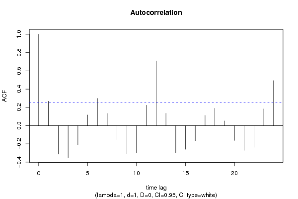
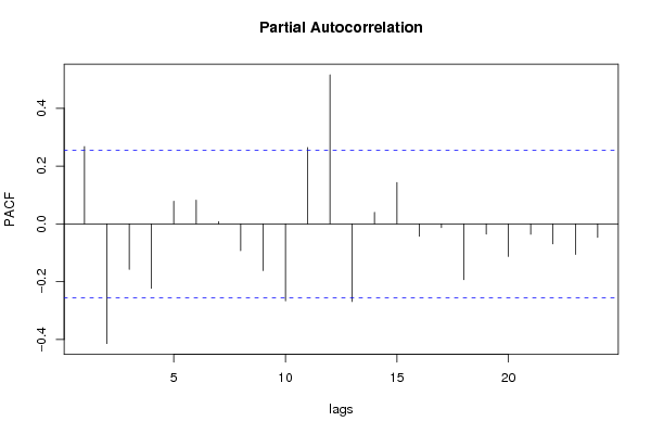
Title produced by software

(Partial) Autocorrelation Function

Date of computation

Fri, 10 Dec 2010 17:26:39 +0000

Cite this page as follows

Statistical Computations at FreeStatistics.org, Office for Research Development and Education, URL https://freestatistics.org/blog/index.php?v=date/2010/Dec/10/t1292001904khn7n1j15hc6p7e.htm/, Retrieved Mon, 29 Apr 2024 08:39:40 +0000

Statistical Computations at FreeStatistics.org, Office for Research Development and Education, URL https://freestatistics.org/blog/index.php?pk=107851, Retrieved Mon, 29 Apr 2024 08:39:40 +0000

QR Codes:

Paste this QR Code to cite your computation.

Original text written by user:

IsPrivate?

No (this computation is public)

User-defined keywords

Estimated Impact

Family? (F = Feedback message, R = changed R code, M = changed R Module, P = changed Parameters, D = changed Data)

-     [(Partial) Autocorrelation Function] [Paper: PACF 1] [2010-12-10 17:20:31] [7d64bf19f34ddcdf2626356c9d5bd60d]
-   P     [(Partial) Autocorrelation Function] [paper ACF 2] [2010-12-10 17:26:39] [5842cf9dd57f9603e676e11284d3404a] [Current]
-   P       [(Partial) Autocorrelation Function] [ACF 3] [2010-12-10 17:29:50] [7d64bf19f34ddcdf2626356c9d5bd60d] 
- R P       [(Partial) Autocorrelation Function] [ACF original] [2010-12-10 17:35:01] [7d64bf19f34ddcdf2626356c9d5bd60d] 
-   P         [(Partial) Autocorrelation Function] [ACF 2] [2010-12-10 17:37:10] [7d64bf19f34ddcdf2626356c9d5bd60d] 
-   P           [(Partial) Autocorrelation Function] [ACF 4] [2010-12-10 17:42:26] [7d64bf19f34ddcdf2626356c9d5bd60d] 

Feedback Forum

Post a new message

Dataseries X:

Download CSV

Histogram

Boxplots

Summary of computational transaction
Raw Input	view raw input (R code)
Raw Output	view raw output of R engine
Computing time	2 seconds
R Server	'Sir Ronald Aylmer Fisher' @ 193.190.124.24

\begin{tabular}{lllllllll}
\hline
Summary of computational transaction \tabularnewline
Raw Input & view raw input (R code)  \tabularnewline
Raw Output & view raw output of R engine  \tabularnewline
Computing time & 2 seconds \tabularnewline
R Server & 'Sir Ronald Aylmer Fisher' @ 193.190.124.24 \tabularnewline
\hline
\end{tabular}
%Source: https://freestatistics.org/blog/index.php?pk=107851&T=0

[TABLE]
[ROW][C]Summary of computational transaction[/C][/ROW]
[ROW][C]Raw Input[/C][C]view raw input (R code) [/C][/ROW]
[ROW][C]Raw Output[/C][C]view raw output of R engine [/C][/ROW]
[ROW][C]Computing time[/C][C]2 seconds[/C][/ROW]
[ROW][C]R Server[/C][C]'Sir Ronald Aylmer Fisher' @ 193.190.124.24[/C][/ROW]
[/TABLE]
Source: https://freestatistics.org/blog/index.php?pk=107851&T=0

Globally Unique Identifier (entire table): ba.freestatistics.org/blog/index.php?pk=107851&T=0

As an alternative you can also use a QR Code:

The GUIDs for individual cells are displayed in the table below:

Summary of computational transaction
Raw Input	view raw input (R code)
Raw Output	view raw output of R engine
Computing time	2 seconds
R Server	'Sir Ronald Aylmer Fisher' @ 193.190.124.24

Autocorrelation Function
Time lag k	ACF(k)	T-STAT	P-value
1	0.267447	2.0543	0.022192
2	-0.312843	-2.403	0.009712
3	-0.349824	-2.687	0.004675
4	-0.208075	-1.5983	0.057665
5	0.117461	0.9022	0.1853
6	0.297746	2.287	0.012899
7	0.132708	1.0193	0.1561
8	-0.152885	-1.1743	0.122491
9	-0.310749	-2.3869	0.010107
10	-0.300084	-2.305	0.012351
11	0.222877	1.7119	0.046079
12	0.709108	5.4468	1e-06
13	0.134791	1.0354	0.152365
14	-0.296722	-2.2792	0.013145
15	-0.258999	-1.9894	0.025649
16	-0.165278	-1.2695	0.10462
17	0.111874	0.8593	0.196822
18	0.189775	1.4577	0.075115
19	0.051717	0.3972	0.346311
20	-0.162997	-1.252	0.107754
21	-0.270745	-2.0796	0.020957
22	-0.237194	-1.8219	0.036768
23	0.184189	1.4148	0.081194
24	0.492579	3.7836	0.000182

\begin{tabular}{lllllllll}
\hline
Autocorrelation Function \tabularnewline
Time lag k & ACF(k) & T-STAT & P-value \tabularnewline
1 & 0.267447 & 2.0543 & 0.022192 \tabularnewline
2 & -0.312843 & -2.403 & 0.009712 \tabularnewline
3 & -0.349824 & -2.687 & 0.004675 \tabularnewline
4 & -0.208075 & -1.5983 & 0.057665 \tabularnewline
5 & 0.117461 & 0.9022 & 0.1853 \tabularnewline
6 & 0.297746 & 2.287 & 0.012899 \tabularnewline
7 & 0.132708 & 1.0193 & 0.1561 \tabularnewline
8 & -0.152885 & -1.1743 & 0.122491 \tabularnewline
9 & -0.310749 & -2.3869 & 0.010107 \tabularnewline
10 & -0.300084 & -2.305 & 0.012351 \tabularnewline
11 & 0.222877 & 1.7119 & 0.046079 \tabularnewline
12 & 0.709108 & 5.4468 & 1e-06 \tabularnewline
13 & 0.134791 & 1.0354 & 0.152365 \tabularnewline
14 & -0.296722 & -2.2792 & 0.013145 \tabularnewline
15 & -0.258999 & -1.9894 & 0.025649 \tabularnewline
16 & -0.165278 & -1.2695 & 0.10462 \tabularnewline
17 & 0.111874 & 0.8593 & 0.196822 \tabularnewline
18 & 0.189775 & 1.4577 & 0.075115 \tabularnewline
19 & 0.051717 & 0.3972 & 0.346311 \tabularnewline
20 & -0.162997 & -1.252 & 0.107754 \tabularnewline
21 & -0.270745 & -2.0796 & 0.020957 \tabularnewline
22 & -0.237194 & -1.8219 & 0.036768 \tabularnewline
23 & 0.184189 & 1.4148 & 0.081194 \tabularnewline
24 & 0.492579 & 3.7836 & 0.000182 \tabularnewline
\hline
\end{tabular}
%Source: https://freestatistics.org/blog/index.php?pk=107851&T=1

[TABLE]
[ROW][C]Autocorrelation Function[/C][/ROW]
[ROW][C]Time lag k[/C][C]ACF(k)[/C][C]T-STAT[/C][C]P-value[/C][/ROW]
[ROW][C]1[/C][C]0.267447[/C][C]2.0543[/C][C]0.022192[/C][/ROW]
[ROW][C]2[/C][C]-0.312843[/C][C]-2.403[/C][C]0.009712[/C][/ROW]
[ROW][C]3[/C][C]-0.349824[/C][C]-2.687[/C][C]0.004675[/C][/ROW]
[ROW][C]4[/C][C]-0.208075[/C][C]-1.5983[/C][C]0.057665[/C][/ROW]
[ROW][C]5[/C][C]0.117461[/C][C]0.9022[/C][C]0.1853[/C][/ROW]
[ROW][C]6[/C][C]0.297746[/C][C]2.287[/C][C]0.012899[/C][/ROW]
[ROW][C]7[/C][C]0.132708[/C][C]1.0193[/C][C]0.1561[/C][/ROW]
[ROW][C]8[/C][C]-0.152885[/C][C]-1.1743[/C][C]0.122491[/C][/ROW]
[ROW][C]9[/C][C]-0.310749[/C][C]-2.3869[/C][C]0.010107[/C][/ROW]
[ROW][C]10[/C][C]-0.300084[/C][C]-2.305[/C][C]0.012351[/C][/ROW]
[ROW][C]11[/C][C]0.222877[/C][C]1.7119[/C][C]0.046079[/C][/ROW]
[ROW][C]12[/C][C]0.709108[/C][C]5.4468[/C][C]1e-06[/C][/ROW]
[ROW][C]13[/C][C]0.134791[/C][C]1.0354[/C][C]0.152365[/C][/ROW]
[ROW][C]14[/C][C]-0.296722[/C][C]-2.2792[/C][C]0.013145[/C][/ROW]
[ROW][C]15[/C][C]-0.258999[/C][C]-1.9894[/C][C]0.025649[/C][/ROW]
[ROW][C]16[/C][C]-0.165278[/C][C]-1.2695[/C][C]0.10462[/C][/ROW]
[ROW][C]17[/C][C]0.111874[/C][C]0.8593[/C][C]0.196822[/C][/ROW]
[ROW][C]18[/C][C]0.189775[/C][C]1.4577[/C][C]0.075115[/C][/ROW]
[ROW][C]19[/C][C]0.051717[/C][C]0.3972[/C][C]0.346311[/C][/ROW]
[ROW][C]20[/C][C]-0.162997[/C][C]-1.252[/C][C]0.107754[/C][/ROW]
[ROW][C]21[/C][C]-0.270745[/C][C]-2.0796[/C][C]0.020957[/C][/ROW]
[ROW][C]22[/C][C]-0.237194[/C][C]-1.8219[/C][C]0.036768[/C][/ROW]
[ROW][C]23[/C][C]0.184189[/C][C]1.4148[/C][C]0.081194[/C][/ROW]
[ROW][C]24[/C][C]0.492579[/C][C]3.7836[/C][C]0.000182[/C][/ROW]
[/TABLE]
Source: https://freestatistics.org/blog/index.php?pk=107851&T=1

Globally Unique Identifier (entire table): ba.freestatistics.org/blog/index.php?pk=107851&T=1

As an alternative you can also use a QR Code:

The GUIDs for individual cells are displayed in the table below:

Autocorrelation Function
Time lag k	ACF(k)	T-STAT	P-value
1	0.267447	2.0543	0.022192
2	-0.312843	-2.403	0.009712
3	-0.349824	-2.687	0.004675
4	-0.208075	-1.5983	0.057665
5	0.117461	0.9022	0.1853
6	0.297746	2.287	0.012899
7	0.132708	1.0193	0.1561
8	-0.152885	-1.1743	0.122491
9	-0.310749	-2.3869	0.010107
10	-0.300084	-2.305	0.012351
11	0.222877	1.7119	0.046079
12	0.709108	5.4468	1e-06
13	0.134791	1.0354	0.152365
14	-0.296722	-2.2792	0.013145
15	-0.258999	-1.9894	0.025649
16	-0.165278	-1.2695	0.10462
17	0.111874	0.8593	0.196822
18	0.189775	1.4577	0.075115
19	0.051717	0.3972	0.346311
20	-0.162997	-1.252	0.107754
21	-0.270745	-2.0796	0.020957
22	-0.237194	-1.8219	0.036768
23	0.184189	1.4148	0.081194
24	0.492579	3.7836	0.000182

Partial Autocorrelation Function
Time lag k	PACF(k)	T-STAT	P-value
1	0.267447	2.0543	0.022192
2	-0.413982	-3.1799	0.001174
3	-0.157015	-1.2061	0.116306
4	-0.223172	-1.7142	0.045869
5	0.078581	0.6036	0.274215
6	0.081801	0.6283	0.266108
7	0.008361	0.0642	0.474505
8	-0.092645	-0.7116	0.239752
9	-0.161507	-1.2406	0.10984
10	-0.266317	-2.0456	0.02263
11	0.26412	2.0287	0.023503
12	0.515732	3.9614	0.000102
13	-0.26853	-2.0626	0.02178
14	0.039983	0.3071	0.379919
15	0.143196	1.0999	0.13792
16	-0.043109	-0.3311	0.370862
17	-0.012583	-0.0966	0.461667
18	-0.193093	-1.4832	0.071675
19	-0.035092	-0.2695	0.394224
20	-0.112788	-0.8663	0.194907
21	-0.035953	-0.2762	0.391696
22	-0.069031	-0.5302	0.298968
23	-0.105906	-0.8135	0.209606
24	-0.046968	-0.3608	0.359781

\begin{tabular}{lllllllll}
\hline
Partial Autocorrelation Function \tabularnewline
Time lag k & PACF(k) & T-STAT & P-value \tabularnewline
1 & 0.267447 & 2.0543 & 0.022192 \tabularnewline
2 & -0.413982 & -3.1799 & 0.001174 \tabularnewline
3 & -0.157015 & -1.2061 & 0.116306 \tabularnewline
4 & -0.223172 & -1.7142 & 0.045869 \tabularnewline
5 & 0.078581 & 0.6036 & 0.274215 \tabularnewline
6 & 0.081801 & 0.6283 & 0.266108 \tabularnewline
7 & 0.008361 & 0.0642 & 0.474505 \tabularnewline
8 & -0.092645 & -0.7116 & 0.239752 \tabularnewline
9 & -0.161507 & -1.2406 & 0.10984 \tabularnewline
10 & -0.266317 & -2.0456 & 0.02263 \tabularnewline
11 & 0.26412 & 2.0287 & 0.023503 \tabularnewline
12 & 0.515732 & 3.9614 & 0.000102 \tabularnewline
13 & -0.26853 & -2.0626 & 0.02178 \tabularnewline
14 & 0.039983 & 0.3071 & 0.379919 \tabularnewline
15 & 0.143196 & 1.0999 & 0.13792 \tabularnewline
16 & -0.043109 & -0.3311 & 0.370862 \tabularnewline
17 & -0.012583 & -0.0966 & 0.461667 \tabularnewline
18 & -0.193093 & -1.4832 & 0.071675 \tabularnewline
19 & -0.035092 & -0.2695 & 0.394224 \tabularnewline
20 & -0.112788 & -0.8663 & 0.194907 \tabularnewline
21 & -0.035953 & -0.2762 & 0.391696 \tabularnewline
22 & -0.069031 & -0.5302 & 0.298968 \tabularnewline
23 & -0.105906 & -0.8135 & 0.209606 \tabularnewline
24 & -0.046968 & -0.3608 & 0.359781 \tabularnewline
\hline
\end{tabular}
%Source: https://freestatistics.org/blog/index.php?pk=107851&T=2

[TABLE]
[ROW][C]Partial Autocorrelation Function[/C][/ROW]
[ROW][C]Time lag k[/C][C]PACF(k)[/C][C]T-STAT[/C][C]P-value[/C][/ROW]
[ROW][C]1[/C][C]0.267447[/C][C]2.0543[/C][C]0.022192[/C][/ROW]
[ROW][C]2[/C][C]-0.413982[/C][C]-3.1799[/C][C]0.001174[/C][/ROW]
[ROW][C]3[/C][C]-0.157015[/C][C]-1.2061[/C][C]0.116306[/C][/ROW]
[ROW][C]4[/C][C]-0.223172[/C][C]-1.7142[/C][C]0.045869[/C][/ROW]
[ROW][C]5[/C][C]0.078581[/C][C]0.6036[/C][C]0.274215[/C][/ROW]
[ROW][C]6[/C][C]0.081801[/C][C]0.6283[/C][C]0.266108[/C][/ROW]
[ROW][C]7[/C][C]0.008361[/C][C]0.0642[/C][C]0.474505[/C][/ROW]
[ROW][C]8[/C][C]-0.092645[/C][C]-0.7116[/C][C]0.239752[/C][/ROW]
[ROW][C]9[/C][C]-0.161507[/C][C]-1.2406[/C][C]0.10984[/C][/ROW]
[ROW][C]10[/C][C]-0.266317[/C][C]-2.0456[/C][C]0.02263[/C][/ROW]
[ROW][C]11[/C][C]0.26412[/C][C]2.0287[/C][C]0.023503[/C][/ROW]
[ROW][C]12[/C][C]0.515732[/C][C]3.9614[/C][C]0.000102[/C][/ROW]
[ROW][C]13[/C][C]-0.26853[/C][C]-2.0626[/C][C]0.02178[/C][/ROW]
[ROW][C]14[/C][C]0.039983[/C][C]0.3071[/C][C]0.379919[/C][/ROW]
[ROW][C]15[/C][C]0.143196[/C][C]1.0999[/C][C]0.13792[/C][/ROW]
[ROW][C]16[/C][C]-0.043109[/C][C]-0.3311[/C][C]0.370862[/C][/ROW]
[ROW][C]17[/C][C]-0.012583[/C][C]-0.0966[/C][C]0.461667[/C][/ROW]
[ROW][C]18[/C][C]-0.193093[/C][C]-1.4832[/C][C]0.071675[/C][/ROW]
[ROW][C]19[/C][C]-0.035092[/C][C]-0.2695[/C][C]0.394224[/C][/ROW]
[ROW][C]20[/C][C]-0.112788[/C][C]-0.8663[/C][C]0.194907[/C][/ROW]
[ROW][C]21[/C][C]-0.035953[/C][C]-0.2762[/C][C]0.391696[/C][/ROW]
[ROW][C]22[/C][C]-0.069031[/C][C]-0.5302[/C][C]0.298968[/C][/ROW]
[ROW][C]23[/C][C]-0.105906[/C][C]-0.8135[/C][C]0.209606[/C][/ROW]
[ROW][C]24[/C][C]-0.046968[/C][C]-0.3608[/C][C]0.359781[/C][/ROW]
[/TABLE]
Source: https://freestatistics.org/blog/index.php?pk=107851&T=2

Globally Unique Identifier (entire table): ba.freestatistics.org/blog/index.php?pk=107851&T=2

As an alternative you can also use a QR Code:

The GUIDs for individual cells are displayed in the table below:

Partial Autocorrelation Function
Time lag k	PACF(k)	T-STAT	P-value
1	0.267447	2.0543	0.022192
2	-0.413982	-3.1799	0.001174
3	-0.157015	-1.2061	0.116306
4	-0.223172	-1.7142	0.045869
5	0.078581	0.6036	0.274215
6	0.081801	0.6283	0.266108
7	0.008361	0.0642	0.474505
8	-0.092645	-0.7116	0.239752
9	-0.161507	-1.2406	0.10984
10	-0.266317	-2.0456	0.02263
11	0.26412	2.0287	0.023503
12	0.515732	3.9614	0.000102
13	-0.26853	-2.0626	0.02178
14	0.039983	0.3071	0.379919
15	0.143196	1.0999	0.13792
16	-0.043109	-0.3311	0.370862
17	-0.012583	-0.0966	0.461667
18	-0.193093	-1.4832	0.071675
19	-0.035092	-0.2695	0.394224
20	-0.112788	-0.8663	0.194907
21	-0.035953	-0.2762	0.391696
22	-0.069031	-0.5302	0.298968
23	-0.105906	-0.8135	0.209606
24	-0.046968	-0.3608	0.359781

Figure 1

PNG link

Postscript link

PDF link

Figure 2

PNG link

Postscript link

PDF link

Parameters (Session):

par1 = 24 ; par2 = 1 ; par3 = 1 ; par4 = 0 ; par5 = 12 ; par6 = White Noise ; par7 = 0.95 ;

Parameters (R input):

par1 = 24 ; par2 = 1 ; par3 = 1 ; par4 = 0 ; par5 = 12 ; par6 = White Noise ; par7 = 0.95 ;

R code (references can be found in the software module):

if (par1 == 'Default') {
par1 = 10*log10(length(x))
} else {
par1 <- as.numeric(par1)
}
par2 <- as.numeric(par2)
par3 <- as.numeric(par3)
par4 <- as.numeric(par4)
par5 <- as.numeric(par5)
if (par6 == 'White Noise') par6 <- 'white' else par6 <- 'ma'
par7 <- as.numeric(par7)
if (par2 == 0) {
x <- log(x)
} else {
x <- (x ^ par2 - 1) / par2
}
if (par3 > 0) x <- diff(x,lag=1,difference=par3)
if (par4 > 0) x <- diff(x,lag=par5,difference=par4)
bitmap(file='pic1.png')
racf <- acf(x, par1, main='Autocorrelation', xlab='time lag', ylab='ACF', ci.type=par6, ci=par7, sub=paste('(lambda=',par2,', d=',par3,', D=',par4,', CI=', par7, ', CI type=',par6,')',sep=''))
dev.off()
bitmap(file='pic2.png')
rpacf <- pacf(x,par1,main='Partial Autocorrelation',xlab='lags',ylab='PACF')
dev.off()
(myacf <- c(racf$acf))
(mypacf <- c(rpacf$acf))
lengthx <- length(x)
sqrtn <- sqrt(lengthx)
load(file='createtable')
a<-table.start()
a<-table.row.start(a)
a<-table.element(a,'Autocorrelation Function',4,TRUE)
a<-table.row.end(a)
a<-table.row.start(a)
a<-table.element(a,'Time lag k',header=TRUE)
a<-table.element(a,hyperlink('basics.htm','ACF(k)','click here for more information about the Autocorrelation Function'),header=TRUE)
a<-table.element(a,'T-STAT',header=TRUE)
a<-table.element(a,'P-value',header=TRUE)
a<-table.row.end(a)
for (i in 2:(par1+1)) {
a<-table.row.start(a)
a<-table.element(a,i-1,header=TRUE)
a<-table.element(a,round(myacf[i],6))
mytstat <- myacf[i]*sqrtn
a<-table.element(a,round(mytstat,4))
a<-table.element(a,round(1-pt(abs(mytstat),lengthx),6))
a<-table.row.end(a)
}
a<-table.end(a)
table.save(a,file='mytable.tab')
a<-table.start()
a<-table.row.start(a)
a<-table.element(a,'Partial Autocorrelation Function',4,TRUE)
a<-table.row.end(a)
a<-table.row.start(a)
a<-table.element(a,'Time lag k',header=TRUE)
a<-table.element(a,hyperlink('basics.htm','PACF(k)','click here for more information about the Partial Autocorrelation Function'),header=TRUE)
a<-table.element(a,'T-STAT',header=TRUE)
a<-table.element(a,'P-value',header=TRUE)
a<-table.row.end(a)
for (i in 1:par1) {
a<-table.row.start(a)
a<-table.element(a,i,header=TRUE)
a<-table.element(a,round(mypacf[i],6))
mytstat <- mypacf[i]*sqrtn
a<-table.element(a,round(mytstat,4))
a<-table.element(a,round(1-pt(abs(mytstat),lengthx),6))
a<-table.row.end(a)
}
a<-table.end(a)
table.save(a,file='mytable1.tab')

Free Statistics

Description of Statistical Computation

Tree of Dependent Computations

Dataset

Tables (Output of Computation)

Figures (Output of Computation)

Input Parameters & R Code