Repository of Reproducible Computations

Free Statistics

of Irreproducible Research!

Author's title

Author

*The author of this computation has been verified*

R Software Module

rwasp_autocorrelation.wasp

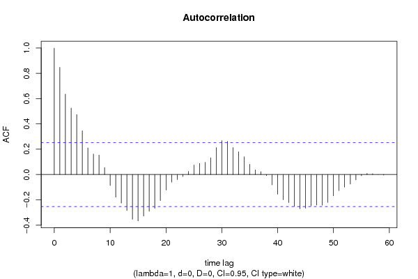
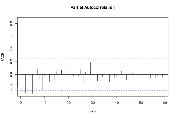
Title produced by software

(Partial) Autocorrelation Function

Date of computation

Fri, 10 Dec 2010 14:01:10 +0000

Cite this page as follows

Statistical Computations at FreeStatistics.org, Office for Research Development and Education, URL https://freestatistics.org/blog/index.php?v=date/2010/Dec/10/t1291989608d4bcve9zz8clc2p.htm/, Retrieved Mon, 29 Apr 2024 10:10:12 +0000

Statistical Computations at FreeStatistics.org, Office for Research Development and Education, URL https://freestatistics.org/blog/index.php?pk=107691, Retrieved Mon, 29 Apr 2024 10:10:12 +0000

QR Codes:

Paste this QR Code to cite your computation.

Original text written by user:

IsPrivate?

No (this computation is public)

User-defined keywords

Estimated Impact

178

Family? (F = Feedback message, R = changed R code, M = changed R Module, P = changed Parameters, D = changed Data)

-     [Univariate Data Series] [] [2008-12-14 11:54:22] [d2d412c7f4d35ffbf5ee5ee89db327d4]
- RMP   [(Partial) Autocorrelation Function] [workshop 9 - 1] [2010-12-03 13:19:03] [ec7b4b7cc1a30b20be5ec01cdf2adbbd]
-   PD      [(Partial) Autocorrelation Function] [paper - time-seri...] [2010-12-10 14:01:10] [6ea41cf020a5319fc3c331a4158019e5] [Current]
-   PD        [(Partial) Autocorrelation Function] [paper - time-seri...] [2010-12-10 15:30:46] [ec7b4b7cc1a30b20be5ec01cdf2adbbd] 
- RMPD        [ARIMA Backward Selection] [paper - time-seri...] [2010-12-10 15:35:16] [ec7b4b7cc1a30b20be5ec01cdf2adbbd] 
- RMPD        [ARIMA Forecasting] [paper - time-seri...] [2010-12-10 15:44:03] [ec7b4b7cc1a30b20be5ec01cdf2adbbd] 
- RMPD        [One-Way-Between-Groups ANOVA- Free Statistics Software (Calculator)] [paper - one-way-a...] [2010-12-15 15:13:20] [ec7b4b7cc1a30b20be5ec01cdf2adbbd] 
-   P           [One-Way-Between-Groups ANOVA- Free Statistics Software (Calculator)] [paper - chi-squared] [2010-12-15 18:25:43] [ec7b4b7cc1a30b20be5ec01cdf2adbbd] 

Feedback Forum

Post a new message

Dataseries X:

Download CSV

Histogram

Boxplots

Summary of computational transaction
Raw Input	view raw input (R code)
Raw Output	view raw output of R engine
Computing time	7 seconds
R Server	'George Udny Yule' @ 72.249.76.132

\begin{tabular}{lllllllll}
\hline
Summary of computational transaction \tabularnewline
Raw Input & view raw input (R code)  \tabularnewline
Raw Output & view raw output of R engine  \tabularnewline
Computing time & 7 seconds \tabularnewline
R Server & 'George Udny Yule' @ 72.249.76.132 \tabularnewline
\hline
\end{tabular}
%Source: https://freestatistics.org/blog/index.php?pk=107691&T=0

[TABLE]
[ROW][C]Summary of computational transaction[/C][/ROW]
[ROW][C]Raw Input[/C][C]view raw input (R code) [/C][/ROW]
[ROW][C]Raw Output[/C][C]view raw output of R engine [/C][/ROW]
[ROW][C]Computing time[/C][C]7 seconds[/C][/ROW]
[ROW][C]R Server[/C][C]'George Udny Yule' @ 72.249.76.132[/C][/ROW]
[/TABLE]
Source: https://freestatistics.org/blog/index.php?pk=107691&T=0

Globally Unique Identifier (entire table): ba.freestatistics.org/blog/index.php?pk=107691&T=0

As an alternative you can also use a QR Code:

The GUIDs for individual cells are displayed in the table below:

Summary of computational transaction
Raw Input	view raw input (R code)
Raw Output	view raw output of R engine
Computing time	7 seconds
R Server	'George Udny Yule' @ 72.249.76.132

Autocorrelation Function
Time lag k	ACF(k)	T-STAT	P-value
1	0.847945	6.5682	0
2	0.636007	4.9265	3e-06
3	0.525772	4.0726	6.9e-05
4	0.473922	3.671	0.000258
5	0.34665	2.6851	0.00468
6	0.210829	1.6331	0.053845
7	0.16237	1.2577	0.106685
8	0.154135	1.1939	0.118603
9	0.05515	0.4272	0.335386
10	-0.086959	-0.6736	0.251581
11	-0.178826	-1.3852	0.085562
12	-0.225736	-1.7485	0.042742
13	-0.284194	-2.2014	0.015784
14	-0.354481	-2.7458	0.003977
15	-0.366352	-2.8378	0.003095
16	-0.328943	-2.548	0.006707
17	-0.290604	-2.251	0.01403
18	-0.267162	-2.0694	0.02141
19	-0.205962	-1.5954	0.057941
20	-0.122843	-0.9515	0.172574
21	-0.060514	-0.4687	0.320477
22	-0.039889	-0.309	0.379205
23	-0.015509	-0.1201	0.45239
24	0.024253	0.1879	0.425809
25	0.075709	0.5864	0.27989
26	0.087932	0.6811	0.249209
27	0.096806	0.7499	0.228136
28	0.132984	1.0301	0.153552
29	0.213574	1.6543	0.051641
30	0.267651	2.0732	0.021227
31	0.262539	2.0336	0.02321
32	0.213859	1.6565	0.051416
33	0.180086	1.3949	0.084088
34	0.140077	1.085	0.141124
35	0.081464	0.631	0.265214
36	0.03772	0.2922	0.385578
37	0.022751	0.1762	0.430353
38	-0.008615	-0.0667	0.473509
39	-0.081496	-0.6313	0.265132
40	-0.156406	-1.2115	0.115224
41	-0.199841	-1.548	0.063446
42	-0.222606	-1.7243	0.044902
43	-0.251224	-1.946	0.028173
44	-0.270981	-2.099	0.020016
45	-0.266787	-2.0665	0.021551
46	-0.248942	-1.9283	0.029277
47	-0.242037	-1.8748	0.032844
48	-0.24245	-1.878	0.032621
49	-0.220337	-1.7067	0.046522
50	-0.16874	-1.3071	0.098091
51	-0.12745	-0.9872	0.163748
52	-0.099519	-0.7709	0.221905
53	-0.075835	-0.5874	0.279565
54	-0.042268	-0.3274	0.372249
55	-0.009125	-0.0707	0.471944
56	0.009543	0.0739	0.470659
57	0.006659	0.0516	0.479518
58	0.000553	0.0043	0.498297
59	-0.004305	-0.0333	0.486754
60	NA	NA	NA

\begin{tabular}{lllllllll}
\hline
Autocorrelation Function \tabularnewline
Time lag k & ACF(k) & T-STAT & P-value \tabularnewline
1 & 0.847945 & 6.5682 & 0 \tabularnewline
2 & 0.636007 & 4.9265 & 3e-06 \tabularnewline
3 & 0.525772 & 4.0726 & 6.9e-05 \tabularnewline
4 & 0.473922 & 3.671 & 0.000258 \tabularnewline
5 & 0.34665 & 2.6851 & 0.00468 \tabularnewline
6 & 0.210829 & 1.6331 & 0.053845 \tabularnewline
7 & 0.16237 & 1.2577 & 0.106685 \tabularnewline
8 & 0.154135 & 1.1939 & 0.118603 \tabularnewline
9 & 0.05515 & 0.4272 & 0.335386 \tabularnewline
10 & -0.086959 & -0.6736 & 0.251581 \tabularnewline
11 & -0.178826 & -1.3852 & 0.085562 \tabularnewline
12 & -0.225736 & -1.7485 & 0.042742 \tabularnewline
13 & -0.284194 & -2.2014 & 0.015784 \tabularnewline
14 & -0.354481 & -2.7458 & 0.003977 \tabularnewline
15 & -0.366352 & -2.8378 & 0.003095 \tabularnewline
16 & -0.328943 & -2.548 & 0.006707 \tabularnewline
17 & -0.290604 & -2.251 & 0.01403 \tabularnewline
18 & -0.267162 & -2.0694 & 0.02141 \tabularnewline
19 & -0.205962 & -1.5954 & 0.057941 \tabularnewline
20 & -0.122843 & -0.9515 & 0.172574 \tabularnewline
21 & -0.060514 & -0.4687 & 0.320477 \tabularnewline
22 & -0.039889 & -0.309 & 0.379205 \tabularnewline
23 & -0.015509 & -0.1201 & 0.45239 \tabularnewline
24 & 0.024253 & 0.1879 & 0.425809 \tabularnewline
25 & 0.075709 & 0.5864 & 0.27989 \tabularnewline
26 & 0.087932 & 0.6811 & 0.249209 \tabularnewline
27 & 0.096806 & 0.7499 & 0.228136 \tabularnewline
28 & 0.132984 & 1.0301 & 0.153552 \tabularnewline
29 & 0.213574 & 1.6543 & 0.051641 \tabularnewline
30 & 0.267651 & 2.0732 & 0.021227 \tabularnewline
31 & 0.262539 & 2.0336 & 0.02321 \tabularnewline
32 & 0.213859 & 1.6565 & 0.051416 \tabularnewline
33 & 0.180086 & 1.3949 & 0.084088 \tabularnewline
34 & 0.140077 & 1.085 & 0.141124 \tabularnewline
35 & 0.081464 & 0.631 & 0.265214 \tabularnewline
36 & 0.03772 & 0.2922 & 0.385578 \tabularnewline
37 & 0.022751 & 0.1762 & 0.430353 \tabularnewline
38 & -0.008615 & -0.0667 & 0.473509 \tabularnewline
39 & -0.081496 & -0.6313 & 0.265132 \tabularnewline
40 & -0.156406 & -1.2115 & 0.115224 \tabularnewline
41 & -0.199841 & -1.548 & 0.063446 \tabularnewline
42 & -0.222606 & -1.7243 & 0.044902 \tabularnewline
43 & -0.251224 & -1.946 & 0.028173 \tabularnewline
44 & -0.270981 & -2.099 & 0.020016 \tabularnewline
45 & -0.266787 & -2.0665 & 0.021551 \tabularnewline
46 & -0.248942 & -1.9283 & 0.029277 \tabularnewline
47 & -0.242037 & -1.8748 & 0.032844 \tabularnewline
48 & -0.24245 & -1.878 & 0.032621 \tabularnewline
49 & -0.220337 & -1.7067 & 0.046522 \tabularnewline
50 & -0.16874 & -1.3071 & 0.098091 \tabularnewline
51 & -0.12745 & -0.9872 & 0.163748 \tabularnewline
52 & -0.099519 & -0.7709 & 0.221905 \tabularnewline
53 & -0.075835 & -0.5874 & 0.279565 \tabularnewline
54 & -0.042268 & -0.3274 & 0.372249 \tabularnewline
55 & -0.009125 & -0.0707 & 0.471944 \tabularnewline
56 & 0.009543 & 0.0739 & 0.470659 \tabularnewline
57 & 0.006659 & 0.0516 & 0.479518 \tabularnewline
58 & 0.000553 & 0.0043 & 0.498297 \tabularnewline
59 & -0.004305 & -0.0333 & 0.486754 \tabularnewline
60 & NA & NA & NA \tabularnewline
\hline
\end{tabular}
%Source: https://freestatistics.org/blog/index.php?pk=107691&T=1

[TABLE]
[ROW][C]Autocorrelation Function[/C][/ROW]
[ROW][C]Time lag k[/C][C]ACF(k)[/C][C]T-STAT[/C][C]P-value[/C][/ROW]
[ROW][C]1[/C][C]0.847945[/C][C]6.5682[/C][C]0[/C][/ROW]
[ROW][C]2[/C][C]0.636007[/C][C]4.9265[/C][C]3e-06[/C][/ROW]
[ROW][C]3[/C][C]0.525772[/C][C]4.0726[/C][C]6.9e-05[/C][/ROW]
[ROW][C]4[/C][C]0.473922[/C][C]3.671[/C][C]0.000258[/C][/ROW]
[ROW][C]5[/C][C]0.34665[/C][C]2.6851[/C][C]0.00468[/C][/ROW]
[ROW][C]6[/C][C]0.210829[/C][C]1.6331[/C][C]0.053845[/C][/ROW]
[ROW][C]7[/C][C]0.16237[/C][C]1.2577[/C][C]0.106685[/C][/ROW]
[ROW][C]8[/C][C]0.154135[/C][C]1.1939[/C][C]0.118603[/C][/ROW]
[ROW][C]9[/C][C]0.05515[/C][C]0.4272[/C][C]0.335386[/C][/ROW]
[ROW][C]10[/C][C]-0.086959[/C][C]-0.6736[/C][C]0.251581[/C][/ROW]
[ROW][C]11[/C][C]-0.178826[/C][C]-1.3852[/C][C]0.085562[/C][/ROW]
[ROW][C]12[/C][C]-0.225736[/C][C]-1.7485[/C][C]0.042742[/C][/ROW]
[ROW][C]13[/C][C]-0.284194[/C][C]-2.2014[/C][C]0.015784[/C][/ROW]
[ROW][C]14[/C][C]-0.354481[/C][C]-2.7458[/C][C]0.003977[/C][/ROW]
[ROW][C]15[/C][C]-0.366352[/C][C]-2.8378[/C][C]0.003095[/C][/ROW]
[ROW][C]16[/C][C]-0.328943[/C][C]-2.548[/C][C]0.006707[/C][/ROW]
[ROW][C]17[/C][C]-0.290604[/C][C]-2.251[/C][C]0.01403[/C][/ROW]
[ROW][C]18[/C][C]-0.267162[/C][C]-2.0694[/C][C]0.02141[/C][/ROW]
[ROW][C]19[/C][C]-0.205962[/C][C]-1.5954[/C][C]0.057941[/C][/ROW]
[ROW][C]20[/C][C]-0.122843[/C][C]-0.9515[/C][C]0.172574[/C][/ROW]
[ROW][C]21[/C][C]-0.060514[/C][C]-0.4687[/C][C]0.320477[/C][/ROW]
[ROW][C]22[/C][C]-0.039889[/C][C]-0.309[/C][C]0.379205[/C][/ROW]
[ROW][C]23[/C][C]-0.015509[/C][C]-0.1201[/C][C]0.45239[/C][/ROW]
[ROW][C]24[/C][C]0.024253[/C][C]0.1879[/C][C]0.425809[/C][/ROW]
[ROW][C]25[/C][C]0.075709[/C][C]0.5864[/C][C]0.27989[/C][/ROW]
[ROW][C]26[/C][C]0.087932[/C][C]0.6811[/C][C]0.249209[/C][/ROW]
[ROW][C]27[/C][C]0.096806[/C][C]0.7499[/C][C]0.228136[/C][/ROW]
[ROW][C]28[/C][C]0.132984[/C][C]1.0301[/C][C]0.153552[/C][/ROW]
[ROW][C]29[/C][C]0.213574[/C][C]1.6543[/C][C]0.051641[/C][/ROW]
[ROW][C]30[/C][C]0.267651[/C][C]2.0732[/C][C]0.021227[/C][/ROW]
[ROW][C]31[/C][C]0.262539[/C][C]2.0336[/C][C]0.02321[/C][/ROW]
[ROW][C]32[/C][C]0.213859[/C][C]1.6565[/C][C]0.051416[/C][/ROW]
[ROW][C]33[/C][C]0.180086[/C][C]1.3949[/C][C]0.084088[/C][/ROW]
[ROW][C]34[/C][C]0.140077[/C][C]1.085[/C][C]0.141124[/C][/ROW]
[ROW][C]35[/C][C]0.081464[/C][C]0.631[/C][C]0.265214[/C][/ROW]
[ROW][C]36[/C][C]0.03772[/C][C]0.2922[/C][C]0.385578[/C][/ROW]
[ROW][C]37[/C][C]0.022751[/C][C]0.1762[/C][C]0.430353[/C][/ROW]
[ROW][C]38[/C][C]-0.008615[/C][C]-0.0667[/C][C]0.473509[/C][/ROW]
[ROW][C]39[/C][C]-0.081496[/C][C]-0.6313[/C][C]0.265132[/C][/ROW]
[ROW][C]40[/C][C]-0.156406[/C][C]-1.2115[/C][C]0.115224[/C][/ROW]
[ROW][C]41[/C][C]-0.199841[/C][C]-1.548[/C][C]0.063446[/C][/ROW]
[ROW][C]42[/C][C]-0.222606[/C][C]-1.7243[/C][C]0.044902[/C][/ROW]
[ROW][C]43[/C][C]-0.251224[/C][C]-1.946[/C][C]0.028173[/C][/ROW]
[ROW][C]44[/C][C]-0.270981[/C][C]-2.099[/C][C]0.020016[/C][/ROW]
[ROW][C]45[/C][C]-0.266787[/C][C]-2.0665[/C][C]0.021551[/C][/ROW]
[ROW][C]46[/C][C]-0.248942[/C][C]-1.9283[/C][C]0.029277[/C][/ROW]
[ROW][C]47[/C][C]-0.242037[/C][C]-1.8748[/C][C]0.032844[/C][/ROW]
[ROW][C]48[/C][C]-0.24245[/C][C]-1.878[/C][C]0.032621[/C][/ROW]
[ROW][C]49[/C][C]-0.220337[/C][C]-1.7067[/C][C]0.046522[/C][/ROW]
[ROW][C]50[/C][C]-0.16874[/C][C]-1.3071[/C][C]0.098091[/C][/ROW]
[ROW][C]51[/C][C]-0.12745[/C][C]-0.9872[/C][C]0.163748[/C][/ROW]
[ROW][C]52[/C][C]-0.099519[/C][C]-0.7709[/C][C]0.221905[/C][/ROW]
[ROW][C]53[/C][C]-0.075835[/C][C]-0.5874[/C][C]0.279565[/C][/ROW]
[ROW][C]54[/C][C]-0.042268[/C][C]-0.3274[/C][C]0.372249[/C][/ROW]
[ROW][C]55[/C][C]-0.009125[/C][C]-0.0707[/C][C]0.471944[/C][/ROW]
[ROW][C]56[/C][C]0.009543[/C][C]0.0739[/C][C]0.470659[/C][/ROW]
[ROW][C]57[/C][C]0.006659[/C][C]0.0516[/C][C]0.479518[/C][/ROW]
[ROW][C]58[/C][C]0.000553[/C][C]0.0043[/C][C]0.498297[/C][/ROW]
[ROW][C]59[/C][C]-0.004305[/C][C]-0.0333[/C][C]0.486754[/C][/ROW]
[ROW][C]60[/C][C]NA[/C][C]NA[/C][C]NA[/C][/ROW]
[/TABLE]
Source: https://freestatistics.org/blog/index.php?pk=107691&T=1

Globally Unique Identifier (entire table): ba.freestatistics.org/blog/index.php?pk=107691&T=1

As an alternative you can also use a QR Code:

The GUIDs for individual cells are displayed in the table below:

Autocorrelation Function
Time lag k	ACF(k)	T-STAT	P-value
1	0.847945	6.5682	0
2	0.636007	4.9265	3e-06
3	0.525772	4.0726	6.9e-05
4	0.473922	3.671	0.000258
5	0.34665	2.6851	0.00468
6	0.210829	1.6331	0.053845
7	0.16237	1.2577	0.106685
8	0.154135	1.1939	0.118603
9	0.05515	0.4272	0.335386
10	-0.086959	-0.6736	0.251581
11	-0.178826	-1.3852	0.085562
12	-0.225736	-1.7485	0.042742
13	-0.284194	-2.2014	0.015784
14	-0.354481	-2.7458	0.003977
15	-0.366352	-2.8378	0.003095
16	-0.328943	-2.548	0.006707
17	-0.290604	-2.251	0.01403
18	-0.267162	-2.0694	0.02141
19	-0.205962	-1.5954	0.057941
20	-0.122843	-0.9515	0.172574
21	-0.060514	-0.4687	0.320477
22	-0.039889	-0.309	0.379205
23	-0.015509	-0.1201	0.45239
24	0.024253	0.1879	0.425809
25	0.075709	0.5864	0.27989
26	0.087932	0.6811	0.249209
27	0.096806	0.7499	0.228136
28	0.132984	1.0301	0.153552
29	0.213574	1.6543	0.051641
30	0.267651	2.0732	0.021227
31	0.262539	2.0336	0.02321
32	0.213859	1.6565	0.051416
33	0.180086	1.3949	0.084088
34	0.140077	1.085	0.141124
35	0.081464	0.631	0.265214
36	0.03772	0.2922	0.385578
37	0.022751	0.1762	0.430353
38	-0.008615	-0.0667	0.473509
39	-0.081496	-0.6313	0.265132
40	-0.156406	-1.2115	0.115224
41	-0.199841	-1.548	0.063446
42	-0.222606	-1.7243	0.044902
43	-0.251224	-1.946	0.028173
44	-0.270981	-2.099	0.020016
45	-0.266787	-2.0665	0.021551
46	-0.248942	-1.9283	0.029277
47	-0.242037	-1.8748	0.032844
48	-0.24245	-1.878	0.032621
49	-0.220337	-1.7067	0.046522
50	-0.16874	-1.3071	0.098091
51	-0.12745	-0.9872	0.163748
52	-0.099519	-0.7709	0.221905
53	-0.075835	-0.5874	0.279565
54	-0.042268	-0.3274	0.372249
55	-0.009125	-0.0707	0.471944
56	0.009543	0.0739	0.470659
57	0.006659	0.0516	0.479518
58	0.000553	0.0043	0.498297
59	-0.004305	-0.0333	0.486754
60	NA	NA	NA

Partial Autocorrelation Function
Time lag k	PACF(k)	T-STAT	P-value
1	0.847945	6.5682	0
2	-0.2954	-2.2882	0.012833
3	0.302755	2.3451	0.011173
4	-0.034168	-0.2647	0.396088
5	-0.297214	-2.3022	0.012405
6	0.125464	0.9718	0.167516
7	0.083989	0.6506	0.258902
8	-0.08716	-0.6751	0.25109
9	-0.244069	-1.8905	0.031758
10	-0.02425	-0.1878	0.425818
11	-0.103218	-0.7995	0.213571
12	-0.110731	-0.8577	0.197231
13	0.034881	0.2702	0.393972
14	-0.08656	-0.6705	0.252558
15	0.044756	0.3467	0.365024
16	-0.008081	-0.0626	0.475149
17	0.069354	0.5372	0.296553
18	0.030201	0.2339	0.407917
19	0.127318	0.9862	0.163998
20	0.00688	0.0533	0.478838
21	-0.004682	-0.0363	0.485594
22	-0.021692	-0.168	0.433564
23	-0.036621	-0.2837	0.388821
24	-0.02869	-0.2222	0.412444
25	0.077654	0.6015	0.274884
26	-0.153926	-1.1923	0.118918
27	0.038305	0.2967	0.383858
28	0.06059	0.4693	0.320269
29	0.188353	1.459	0.074894
30	0.002623	0.0203	0.491929
31	-0.014071	-0.109	0.456787
32	-0.098185	-0.7605	0.224955
33	-0.005561	-0.0431	0.482892
34	-0.039587	-0.3066	0.380089
35	0.012588	0.0975	0.461324
36	0.063963	0.4955	0.311044
37	-0.113848	-0.8819	0.190686
38	-0.168402	-1.3044	0.098534
39	-0.046941	-0.3636	0.358716
40	-0.032553	-0.2522	0.400893
41	0.001885	0.0146	0.494201
42	0.050845	0.3938	0.347545
43	0.058262	0.4513	0.326701
44	-0.080023	-0.6199	0.268849
45	0.033046	0.256	0.399425
46	0.029712	0.2301	0.409379
47	0.02409	0.1866	0.426303
48	-0.078294	-0.6065	0.273248
49	0.004835	0.0374	0.485126
50	-0.057577	-0.446	0.328606
51	-0.060269	-0.4668	0.321152
52	0.009472	0.0734	0.470879
53	-0.062774	-0.4862	0.314281
54	-0.055285	-0.4282	0.335007
55	0.024192	0.1874	0.425993
56	-0.050065	-0.3878	0.349769
57	-0.017716	-0.1372	0.445654
58	-0.031561	-0.2445	0.40385
59	-0.039347	-0.3048	0.380795
60	NA	NA	NA

\begin{tabular}{lllllllll}
\hline
Partial Autocorrelation Function \tabularnewline
Time lag k & PACF(k) & T-STAT & P-value \tabularnewline
1 & 0.847945 & 6.5682 & 0 \tabularnewline
2 & -0.2954 & -2.2882 & 0.012833 \tabularnewline
3 & 0.302755 & 2.3451 & 0.011173 \tabularnewline
4 & -0.034168 & -0.2647 & 0.396088 \tabularnewline
5 & -0.297214 & -2.3022 & 0.012405 \tabularnewline
6 & 0.125464 & 0.9718 & 0.167516 \tabularnewline
7 & 0.083989 & 0.6506 & 0.258902 \tabularnewline
8 & -0.08716 & -0.6751 & 0.25109 \tabularnewline
9 & -0.244069 & -1.8905 & 0.031758 \tabularnewline
10 & -0.02425 & -0.1878 & 0.425818 \tabularnewline
11 & -0.103218 & -0.7995 & 0.213571 \tabularnewline
12 & -0.110731 & -0.8577 & 0.197231 \tabularnewline
13 & 0.034881 & 0.2702 & 0.393972 \tabularnewline
14 & -0.08656 & -0.6705 & 0.252558 \tabularnewline
15 & 0.044756 & 0.3467 & 0.365024 \tabularnewline
16 & -0.008081 & -0.0626 & 0.475149 \tabularnewline
17 & 0.069354 & 0.5372 & 0.296553 \tabularnewline
18 & 0.030201 & 0.2339 & 0.407917 \tabularnewline
19 & 0.127318 & 0.9862 & 0.163998 \tabularnewline
20 & 0.00688 & 0.0533 & 0.478838 \tabularnewline
21 & -0.004682 & -0.0363 & 0.485594 \tabularnewline
22 & -0.021692 & -0.168 & 0.433564 \tabularnewline
23 & -0.036621 & -0.2837 & 0.388821 \tabularnewline
24 & -0.02869 & -0.2222 & 0.412444 \tabularnewline
25 & 0.077654 & 0.6015 & 0.274884 \tabularnewline
26 & -0.153926 & -1.1923 & 0.118918 \tabularnewline
27 & 0.038305 & 0.2967 & 0.383858 \tabularnewline
28 & 0.06059 & 0.4693 & 0.320269 \tabularnewline
29 & 0.188353 & 1.459 & 0.074894 \tabularnewline
30 & 0.002623 & 0.0203 & 0.491929 \tabularnewline
31 & -0.014071 & -0.109 & 0.456787 \tabularnewline
32 & -0.098185 & -0.7605 & 0.224955 \tabularnewline
33 & -0.005561 & -0.0431 & 0.482892 \tabularnewline
34 & -0.039587 & -0.3066 & 0.380089 \tabularnewline
35 & 0.012588 & 0.0975 & 0.461324 \tabularnewline
36 & 0.063963 & 0.4955 & 0.311044 \tabularnewline
37 & -0.113848 & -0.8819 & 0.190686 \tabularnewline
38 & -0.168402 & -1.3044 & 0.098534 \tabularnewline
39 & -0.046941 & -0.3636 & 0.358716 \tabularnewline
40 & -0.032553 & -0.2522 & 0.400893 \tabularnewline
41 & 0.001885 & 0.0146 & 0.494201 \tabularnewline
42 & 0.050845 & 0.3938 & 0.347545 \tabularnewline
43 & 0.058262 & 0.4513 & 0.326701 \tabularnewline
44 & -0.080023 & -0.6199 & 0.268849 \tabularnewline
45 & 0.033046 & 0.256 & 0.399425 \tabularnewline
46 & 0.029712 & 0.2301 & 0.409379 \tabularnewline
47 & 0.02409 & 0.1866 & 0.426303 \tabularnewline
48 & -0.078294 & -0.6065 & 0.273248 \tabularnewline
49 & 0.004835 & 0.0374 & 0.485126 \tabularnewline
50 & -0.057577 & -0.446 & 0.328606 \tabularnewline
51 & -0.060269 & -0.4668 & 0.321152 \tabularnewline
52 & 0.009472 & 0.0734 & 0.470879 \tabularnewline
53 & -0.062774 & -0.4862 & 0.314281 \tabularnewline
54 & -0.055285 & -0.4282 & 0.335007 \tabularnewline
55 & 0.024192 & 0.1874 & 0.425993 \tabularnewline
56 & -0.050065 & -0.3878 & 0.349769 \tabularnewline
57 & -0.017716 & -0.1372 & 0.445654 \tabularnewline
58 & -0.031561 & -0.2445 & 0.40385 \tabularnewline
59 & -0.039347 & -0.3048 & 0.380795 \tabularnewline
60 & NA & NA & NA \tabularnewline
\hline
\end{tabular}
%Source: https://freestatistics.org/blog/index.php?pk=107691&T=2

[TABLE]
[ROW][C]Partial Autocorrelation Function[/C][/ROW]
[ROW][C]Time lag k[/C][C]PACF(k)[/C][C]T-STAT[/C][C]P-value[/C][/ROW]
[ROW][C]1[/C][C]0.847945[/C][C]6.5682[/C][C]0[/C][/ROW]
[ROW][C]2[/C][C]-0.2954[/C][C]-2.2882[/C][C]0.012833[/C][/ROW]
[ROW][C]3[/C][C]0.302755[/C][C]2.3451[/C][C]0.011173[/C][/ROW]
[ROW][C]4[/C][C]-0.034168[/C][C]-0.2647[/C][C]0.396088[/C][/ROW]
[ROW][C]5[/C][C]-0.297214[/C][C]-2.3022[/C][C]0.012405[/C][/ROW]
[ROW][C]6[/C][C]0.125464[/C][C]0.9718[/C][C]0.167516[/C][/ROW]
[ROW][C]7[/C][C]0.083989[/C][C]0.6506[/C][C]0.258902[/C][/ROW]
[ROW][C]8[/C][C]-0.08716[/C][C]-0.6751[/C][C]0.25109[/C][/ROW]
[ROW][C]9[/C][C]-0.244069[/C][C]-1.8905[/C][C]0.031758[/C][/ROW]
[ROW][C]10[/C][C]-0.02425[/C][C]-0.1878[/C][C]0.425818[/C][/ROW]
[ROW][C]11[/C][C]-0.103218[/C][C]-0.7995[/C][C]0.213571[/C][/ROW]
[ROW][C]12[/C][C]-0.110731[/C][C]-0.8577[/C][C]0.197231[/C][/ROW]
[ROW][C]13[/C][C]0.034881[/C][C]0.2702[/C][C]0.393972[/C][/ROW]
[ROW][C]14[/C][C]-0.08656[/C][C]-0.6705[/C][C]0.252558[/C][/ROW]
[ROW][C]15[/C][C]0.044756[/C][C]0.3467[/C][C]0.365024[/C][/ROW]
[ROW][C]16[/C][C]-0.008081[/C][C]-0.0626[/C][C]0.475149[/C][/ROW]
[ROW][C]17[/C][C]0.069354[/C][C]0.5372[/C][C]0.296553[/C][/ROW]
[ROW][C]18[/C][C]0.030201[/C][C]0.2339[/C][C]0.407917[/C][/ROW]
[ROW][C]19[/C][C]0.127318[/C][C]0.9862[/C][C]0.163998[/C][/ROW]
[ROW][C]20[/C][C]0.00688[/C][C]0.0533[/C][C]0.478838[/C][/ROW]
[ROW][C]21[/C][C]-0.004682[/C][C]-0.0363[/C][C]0.485594[/C][/ROW]
[ROW][C]22[/C][C]-0.021692[/C][C]-0.168[/C][C]0.433564[/C][/ROW]
[ROW][C]23[/C][C]-0.036621[/C][C]-0.2837[/C][C]0.388821[/C][/ROW]
[ROW][C]24[/C][C]-0.02869[/C][C]-0.2222[/C][C]0.412444[/C][/ROW]
[ROW][C]25[/C][C]0.077654[/C][C]0.6015[/C][C]0.274884[/C][/ROW]
[ROW][C]26[/C][C]-0.153926[/C][C]-1.1923[/C][C]0.118918[/C][/ROW]
[ROW][C]27[/C][C]0.038305[/C][C]0.2967[/C][C]0.383858[/C][/ROW]
[ROW][C]28[/C][C]0.06059[/C][C]0.4693[/C][C]0.320269[/C][/ROW]
[ROW][C]29[/C][C]0.188353[/C][C]1.459[/C][C]0.074894[/C][/ROW]
[ROW][C]30[/C][C]0.002623[/C][C]0.0203[/C][C]0.491929[/C][/ROW]
[ROW][C]31[/C][C]-0.014071[/C][C]-0.109[/C][C]0.456787[/C][/ROW]
[ROW][C]32[/C][C]-0.098185[/C][C]-0.7605[/C][C]0.224955[/C][/ROW]
[ROW][C]33[/C][C]-0.005561[/C][C]-0.0431[/C][C]0.482892[/C][/ROW]
[ROW][C]34[/C][C]-0.039587[/C][C]-0.3066[/C][C]0.380089[/C][/ROW]
[ROW][C]35[/C][C]0.012588[/C][C]0.0975[/C][C]0.461324[/C][/ROW]
[ROW][C]36[/C][C]0.063963[/C][C]0.4955[/C][C]0.311044[/C][/ROW]
[ROW][C]37[/C][C]-0.113848[/C][C]-0.8819[/C][C]0.190686[/C][/ROW]
[ROW][C]38[/C][C]-0.168402[/C][C]-1.3044[/C][C]0.098534[/C][/ROW]
[ROW][C]39[/C][C]-0.046941[/C][C]-0.3636[/C][C]0.358716[/C][/ROW]
[ROW][C]40[/C][C]-0.032553[/C][C]-0.2522[/C][C]0.400893[/C][/ROW]
[ROW][C]41[/C][C]0.001885[/C][C]0.0146[/C][C]0.494201[/C][/ROW]
[ROW][C]42[/C][C]0.050845[/C][C]0.3938[/C][C]0.347545[/C][/ROW]
[ROW][C]43[/C][C]0.058262[/C][C]0.4513[/C][C]0.326701[/C][/ROW]
[ROW][C]44[/C][C]-0.080023[/C][C]-0.6199[/C][C]0.268849[/C][/ROW]
[ROW][C]45[/C][C]0.033046[/C][C]0.256[/C][C]0.399425[/C][/ROW]
[ROW][C]46[/C][C]0.029712[/C][C]0.2301[/C][C]0.409379[/C][/ROW]
[ROW][C]47[/C][C]0.02409[/C][C]0.1866[/C][C]0.426303[/C][/ROW]
[ROW][C]48[/C][C]-0.078294[/C][C]-0.6065[/C][C]0.273248[/C][/ROW]
[ROW][C]49[/C][C]0.004835[/C][C]0.0374[/C][C]0.485126[/C][/ROW]
[ROW][C]50[/C][C]-0.057577[/C][C]-0.446[/C][C]0.328606[/C][/ROW]
[ROW][C]51[/C][C]-0.060269[/C][C]-0.4668[/C][C]0.321152[/C][/ROW]
[ROW][C]52[/C][C]0.009472[/C][C]0.0734[/C][C]0.470879[/C][/ROW]
[ROW][C]53[/C][C]-0.062774[/C][C]-0.4862[/C][C]0.314281[/C][/ROW]
[ROW][C]54[/C][C]-0.055285[/C][C]-0.4282[/C][C]0.335007[/C][/ROW]
[ROW][C]55[/C][C]0.024192[/C][C]0.1874[/C][C]0.425993[/C][/ROW]
[ROW][C]56[/C][C]-0.050065[/C][C]-0.3878[/C][C]0.349769[/C][/ROW]
[ROW][C]57[/C][C]-0.017716[/C][C]-0.1372[/C][C]0.445654[/C][/ROW]
[ROW][C]58[/C][C]-0.031561[/C][C]-0.2445[/C][C]0.40385[/C][/ROW]
[ROW][C]59[/C][C]-0.039347[/C][C]-0.3048[/C][C]0.380795[/C][/ROW]
[ROW][C]60[/C][C]NA[/C][C]NA[/C][C]NA[/C][/ROW]
[/TABLE]
Source: https://freestatistics.org/blog/index.php?pk=107691&T=2

Globally Unique Identifier (entire table): ba.freestatistics.org/blog/index.php?pk=107691&T=2

As an alternative you can also use a QR Code:

The GUIDs for individual cells are displayed in the table below:

Partial Autocorrelation Function
Time lag k	PACF(k)	T-STAT	P-value
1	0.847945	6.5682	0
2	-0.2954	-2.2882	0.012833
3	0.302755	2.3451	0.011173
4	-0.034168	-0.2647	0.396088
5	-0.297214	-2.3022	0.012405
6	0.125464	0.9718	0.167516
7	0.083989	0.6506	0.258902
8	-0.08716	-0.6751	0.25109
9	-0.244069	-1.8905	0.031758
10	-0.02425	-0.1878	0.425818
11	-0.103218	-0.7995	0.213571
12	-0.110731	-0.8577	0.197231
13	0.034881	0.2702	0.393972
14	-0.08656	-0.6705	0.252558
15	0.044756	0.3467	0.365024
16	-0.008081	-0.0626	0.475149
17	0.069354	0.5372	0.296553
18	0.030201	0.2339	0.407917
19	0.127318	0.9862	0.163998
20	0.00688	0.0533	0.478838
21	-0.004682	-0.0363	0.485594
22	-0.021692	-0.168	0.433564
23	-0.036621	-0.2837	0.388821
24	-0.02869	-0.2222	0.412444
25	0.077654	0.6015	0.274884
26	-0.153926	-1.1923	0.118918
27	0.038305	0.2967	0.383858
28	0.06059	0.4693	0.320269
29	0.188353	1.459	0.074894
30	0.002623	0.0203	0.491929
31	-0.014071	-0.109	0.456787
32	-0.098185	-0.7605	0.224955
33	-0.005561	-0.0431	0.482892
34	-0.039587	-0.3066	0.380089
35	0.012588	0.0975	0.461324
36	0.063963	0.4955	0.311044
37	-0.113848	-0.8819	0.190686
38	-0.168402	-1.3044	0.098534
39	-0.046941	-0.3636	0.358716
40	-0.032553	-0.2522	0.400893
41	0.001885	0.0146	0.494201
42	0.050845	0.3938	0.347545
43	0.058262	0.4513	0.326701
44	-0.080023	-0.6199	0.268849
45	0.033046	0.256	0.399425
46	0.029712	0.2301	0.409379
47	0.02409	0.1866	0.426303
48	-0.078294	-0.6065	0.273248
49	0.004835	0.0374	0.485126
50	-0.057577	-0.446	0.328606
51	-0.060269	-0.4668	0.321152
52	0.009472	0.0734	0.470879
53	-0.062774	-0.4862	0.314281
54	-0.055285	-0.4282	0.335007
55	0.024192	0.1874	0.425993
56	-0.050065	-0.3878	0.349769
57	-0.017716	-0.1372	0.445654
58	-0.031561	-0.2445	0.40385
59	-0.039347	-0.3048	0.380795
60	NA	NA	NA

Figure 1

PNG link

Postscript link

PDF link

Figure 2

PNG link

Postscript link

PDF link

Parameters (Session):

par1 = 60 ; par2 = 1 ; par3 = 0 ; par4 = 0 ; par5 = 4 ; par6 = White Noise ; par7 = 0.95 ;

Parameters (R input):

par1 = 60 ; par2 = 1 ; par3 = 0 ; par4 = 0 ; par5 = 4 ; par6 = White Noise ; par7 = 0.95 ;

R code (references can be found in the software module):

if (par1 == 'Default') {
par1 = 10*log10(length(x))
} else {
par1 <- as.numeric(par1)
}
par2 <- as.numeric(par2)
par3 <- as.numeric(par3)
par4 <- as.numeric(par4)
par5 <- as.numeric(par5)
if (par6 == 'White Noise') par6 <- 'white' else par6 <- 'ma'
par7 <- as.numeric(par7)
if (par2 == 0) {
x <- log(x)
} else {
x <- (x ^ par2 - 1) / par2
}
if (par3 > 0) x <- diff(x,lag=1,difference=par3)
if (par4 > 0) x <- diff(x,lag=par5,difference=par4)
bitmap(file='pic1.png')
racf <- acf(x, par1, main='Autocorrelation', xlab='time lag', ylab='ACF', ci.type=par6, ci=par7, sub=paste('(lambda=',par2,', d=',par3,', D=',par4,', CI=', par7, ', CI type=',par6,')',sep=''))
dev.off()
bitmap(file='pic2.png')
rpacf <- pacf(x,par1,main='Partial Autocorrelation',xlab='lags',ylab='PACF')
dev.off()
(myacf <- c(racf$acf))
(mypacf <- c(rpacf$acf))
lengthx <- length(x)
sqrtn <- sqrt(lengthx)
load(file='createtable')
a<-table.start()
a<-table.row.start(a)
a<-table.element(a,'Autocorrelation Function',4,TRUE)
a<-table.row.end(a)
a<-table.row.start(a)
a<-table.element(a,'Time lag k',header=TRUE)
a<-table.element(a,hyperlink('basics.htm','ACF(k)','click here for more information about the Autocorrelation Function'),header=TRUE)
a<-table.element(a,'T-STAT',header=TRUE)
a<-table.element(a,'P-value',header=TRUE)
a<-table.row.end(a)
for (i in 2:(par1+1)) {
a<-table.row.start(a)
a<-table.element(a,i-1,header=TRUE)
a<-table.element(a,round(myacf[i],6))
mytstat <- myacf[i]*sqrtn
a<-table.element(a,round(mytstat,4))
a<-table.element(a,round(1-pt(abs(mytstat),lengthx),6))
a<-table.row.end(a)
}
a<-table.end(a)
table.save(a,file='mytable.tab')
a<-table.start()
a<-table.row.start(a)
a<-table.element(a,'Partial Autocorrelation Function',4,TRUE)
a<-table.row.end(a)
a<-table.row.start(a)
a<-table.element(a,'Time lag k',header=TRUE)
a<-table.element(a,hyperlink('basics.htm','PACF(k)','click here for more information about the Partial Autocorrelation Function'),header=TRUE)
a<-table.element(a,'T-STAT',header=TRUE)
a<-table.element(a,'P-value',header=TRUE)
a<-table.row.end(a)
for (i in 1:par1) {
a<-table.row.start(a)
a<-table.element(a,i,header=TRUE)
a<-table.element(a,round(mypacf[i],6))
mytstat <- mypacf[i]*sqrtn
a<-table.element(a,round(mytstat,4))
a<-table.element(a,round(1-pt(abs(mytstat),lengthx),6))
a<-table.row.end(a)
}
a<-table.end(a)
table.save(a,file='mytable1.tab')

Free Statistics

Description of Statistical Computation

Tree of Dependent Computations

Dataset

Tables (Output of Computation)

Figures (Output of Computation)

Input Parameters & R Code