Repository of Reproducible Computations

Free Statistics

of Irreproducible Research!

Author's title

Author

*The author of this computation has been verified*

R Software Module

rwasp_pairs.wasp

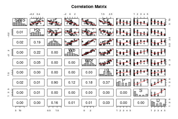
Title produced by software

Kendall tau Correlation Matrix

Date of computation

Fri, 10 Dec 2010 12:15:36 +0000

Cite this page as follows

Statistical Computations at FreeStatistics.org, Office for Research Development and Education, URL https://freestatistics.org/blog/index.php?v=date/2010/Dec/10/t1291983335sfnh6m7limu6c4b.htm/, Retrieved Mon, 29 Apr 2024 11:46:35 +0000

Statistical Computations at FreeStatistics.org, Office for Research Development and Education, URL https://freestatistics.org/blog/index.php?pk=107598, Retrieved Mon, 29 Apr 2024 11:46:35 +0000

QR Codes:

Paste this QR Code to cite your computation.

Original text written by user:

IsPrivate?

No (this computation is public)

User-defined keywords

Estimated Impact

134

Family? (F = Feedback message, R = changed R code, M = changed R Module, P = changed Parameters, D = changed Data)

-       [Kendall tau Correlation Matrix] [science paper] [2010-12-10 12:15:36] [de8ccb310fbbdc3d90ae577a3e011cf9] [Current]
-    D    [Kendall tau Correlation Matrix] [Science paper cor...] [2010-12-10 13:26:41] [04d4386fa51dbd2ef12d0f1f80644886] 
-   PD      [Kendall tau Correlation Matrix] [science paper matrix] [2010-12-10 14:14:21] [04d4386fa51dbd2ef12d0f1f80644886] 
- RMPD    [Multiple Regression] [science paper mul...] [2010-12-10 13:51:45] [04d4386fa51dbd2ef12d0f1f80644886] 
-   PD      [Multiple Regression] [Science paper mr 1] [2010-12-10 14:17:17] [04d4386fa51dbd2ef12d0f1f80644886] 
- RMPD    [Multiple Regression] [science paper mul...] [2010-12-10 14:01:32] [04d4386fa51dbd2ef12d0f1f80644886] 
-    D      [Multiple Regression] [science paper mr 2] [2010-12-10 14:20:17] [04d4386fa51dbd2ef12d0f1f80644886] 

Feedback Forum

Post a new message

Dataseries X:

Download CSV

Histogram

Boxplots

6,3	0,3	0,65	0	0,82	1,62	3	1	3
2,1	0,26	1,84	3,41	3,66	2,8	3	5	4
9,1	-0,15	1,43	1,02	2,25	2,26	4	4	4
15,8	0,59	1,28	-1,64	-0,52	1,54	1	1	1
5,2	0	1,48	2,2	2,23	2,59	4	5	4
10,9	0,56	1,45	0,52	1,41	1,8	1	2	1
8,3	0,15	1,7	1,72	2,64	2,36	1	1	1
11	0,18	0,85	-0,37	0,81	2,05	5	4	4
3,2	-0,15	1,48	2,67	2,63	2,45	5	5	5
6,3	0,32	0,54	-1,12	0,08	1,62	1	1	1
6,6	0,61	0,78	-0,11	0,54	1,62	2	2	2
9,5	0,08	1,02	-0,7	0,7	2,08	2	2	2
3,3	-0,3	1,3	1,44	2,06	2,17	5	5	5
11	0,53	0,59	-0,92	0	1,2	3	1	2
4,7	0,18	1,61	1,93	2,51	2,49	1	3	1
10,4	0,53	0,95	-1	0,6	1,45	5	1	3
7,4	-0,1	0,88	0,02	0,74	1,83	5	3	4
2,1	0,9	1,66	2,72	2,82	2,53	5	5	5
17,9	0,3	1,38	-2	-0,6	1,7	1	1	1
6,1	0,28	2	1,79	3,12	2,43	1	1	1
11,9	0,11	0,51	-1,64	-0,4	1,28	4	1	3
13,8	0,75	0,7	0,23	0,8	1,08	2	1	1
14,3	0,49	0,81	0,54	1,03	2,08	2	1	1
15,2	0,26	1,08	-0,32	1,19	2,15	2	2	2
10	-0,05	1,31	1	2,06	2,23	4	4	4
11,9	0,26	1,11	0,21	1,06	1,23	2	1	2
6,5	0,28	1,43	2,28	2,26	2,06	4	4	4
7,5	-0,05	1,26	0,4	1,08	1,49	5	5	5
10,6	0,41	0,67	-0,55	0,28	1,32	3	1	3
7,4	0,38	0,99	0,63	1,7	1,72	1	1	1
8,4	0,08	1,46	0,83	2,25	2,21	2	3	2
5,7	-0,05	0,85	-0,12	1,09	2,35	2	2	2
4,9	-0,3	0,78	0,56	1,32	2,35	3	2	3
3,2	-0,22	1,3	1,74	3,24	2,18	5	5	5
11	0,36	0,65	-0,05	0,41	1,78	2	1	2
4,9	-0,3	0,88	0,3	1,09	2,3	3	1	3
13,2	0,41	0,36	-0,98	0,4	1,66	3	2	2
9,7	-0,22	1,38	0,62	1,76	2,32	4	3	4
12,8	0,82	0,48	0,54	0,59	1,15	2	1	1

Summary of computational transaction
Raw Input	view raw input (R code)
Raw Output	view raw output of R engine
Computing time	2 seconds
R Server	'RServer@AstonUniversity' @ vre.aston.ac.uk

\begin{tabular}{lllllllll}
\hline
Summary of computational transaction \tabularnewline
Raw Input & view raw input (R code)  \tabularnewline
Raw Output & view raw output of R engine  \tabularnewline
Computing time & 2 seconds \tabularnewline
R Server & 'RServer@AstonUniversity' @ vre.aston.ac.uk \tabularnewline
\hline
\end{tabular}
%Source: https://freestatistics.org/blog/index.php?pk=107598&T=0

[TABLE]
[ROW][C]Summary of computational transaction[/C][/ROW]
[ROW][C]Raw Input[/C][C]view raw input (R code) [/C][/ROW]
[ROW][C]Raw Output[/C][C]view raw output of R engine [/C][/ROW]
[ROW][C]Computing time[/C][C]2 seconds[/C][/ROW]
[ROW][C]R Server[/C][C]'RServer@AstonUniversity' @ vre.aston.ac.uk[/C][/ROW]
[/TABLE]
Source: https://freestatistics.org/blog/index.php?pk=107598&T=0

Globally Unique Identifier (entire table): ba.freestatistics.org/blog/index.php?pk=107598&T=0

As an alternative you can also use a QR Code:

The GUIDs for individual cells are displayed in the table below:

Summary of computational transaction
Raw Input	view raw input (R code)
Raw Output	view raw output of R engine
Computing time	2 seconds
R Server	'RServer@AstonUniversity' @ vre.aston.ac.uk

Correlations for all pairs of data series (method=pearson)
	SWS	PS	L	Wb	Wbr	Tg	P	S	D
SWS	1	0.412	-0.378	-0.712	-0.691	-0.601	-0.369	-0.58	-0.542
PS	0.412	1	-0.213	-0.203	-0.313	-0.5	-0.387	-0.422	-0.513
L	-0.378	-0.213	1	0.684	0.763	0.681	0.02	0.52	0.228
Wb	-0.712	-0.203	0.684	1	0.938	0.696	0.253	0.662	0.432
Wbr	-0.691	-0.313	0.763	0.938	1	0.766	0.221	0.644	0.405
Tg	-0.601	-0.5	0.681	0.696	0.766	1	0.148	0.58	0.354
P	-0.369	-0.387	0.02	0.253	0.221	0.148	1	0.68	0.93
S	-0.58	-0.422	0.52	0.662	0.644	0.58	0.68	1	0.819
D	-0.542	-0.513	0.228	0.432	0.405	0.354	0.93	0.819	1

\begin{tabular}{lllllllll}
\hline
Correlations for all pairs of data series (method=pearson) \tabularnewline
  & SWS & PS & L & Wb & Wbr & Tg & P & S & D \tabularnewline
SWS & 1 & 0.412 & -0.378 & -0.712 & -0.691 & -0.601 & -0.369 & -0.58 & -0.542 \tabularnewline
PS & 0.412 & 1 & -0.213 & -0.203 & -0.313 & -0.5 & -0.387 & -0.422 & -0.513 \tabularnewline
L & -0.378 & -0.213 & 1 & 0.684 & 0.763 & 0.681 & 0.02 & 0.52 & 0.228 \tabularnewline
Wb & -0.712 & -0.203 & 0.684 & 1 & 0.938 & 0.696 & 0.253 & 0.662 & 0.432 \tabularnewline
Wbr & -0.691 & -0.313 & 0.763 & 0.938 & 1 & 0.766 & 0.221 & 0.644 & 0.405 \tabularnewline
Tg & -0.601 & -0.5 & 0.681 & 0.696 & 0.766 & 1 & 0.148 & 0.58 & 0.354 \tabularnewline
P & -0.369 & -0.387 & 0.02 & 0.253 & 0.221 & 0.148 & 1 & 0.68 & 0.93 \tabularnewline
S & -0.58 & -0.422 & 0.52 & 0.662 & 0.644 & 0.58 & 0.68 & 1 & 0.819 \tabularnewline
D & -0.542 & -0.513 & 0.228 & 0.432 & 0.405 & 0.354 & 0.93 & 0.819 & 1 \tabularnewline
\hline
\end{tabular}
%Source: https://freestatistics.org/blog/index.php?pk=107598&T=1

[TABLE]
[ROW][C]Correlations for all pairs of data series (method=pearson)[/C][/ROW]
[ROW][C] [/C][C]SWS[/C][C]PS[/C][C]L[/C][C]Wb[/C][C]Wbr[/C][C]Tg[/C][C]P[/C][C]S[/C][C]D[/C][/ROW]
[ROW][C]SWS[/C][C]1[/C][C]0.412[/C][C]-0.378[/C][C]-0.712[/C][C]-0.691[/C][C]-0.601[/C][C]-0.369[/C][C]-0.58[/C][C]-0.542[/C][/ROW]
[ROW][C]PS[/C][C]0.412[/C][C]1[/C][C]-0.213[/C][C]-0.203[/C][C]-0.313[/C][C]-0.5[/C][C]-0.387[/C][C]-0.422[/C][C]-0.513[/C][/ROW]
[ROW][C]L[/C][C]-0.378[/C][C]-0.213[/C][C]1[/C][C]0.684[/C][C]0.763[/C][C]0.681[/C][C]0.02[/C][C]0.52[/C][C]0.228[/C][/ROW]
[ROW][C]Wb[/C][C]-0.712[/C][C]-0.203[/C][C]0.684[/C][C]1[/C][C]0.938[/C][C]0.696[/C][C]0.253[/C][C]0.662[/C][C]0.432[/C][/ROW]
[ROW][C]Wbr[/C][C]-0.691[/C][C]-0.313[/C][C]0.763[/C][C]0.938[/C][C]1[/C][C]0.766[/C][C]0.221[/C][C]0.644[/C][C]0.405[/C][/ROW]
[ROW][C]Tg[/C][C]-0.601[/C][C]-0.5[/C][C]0.681[/C][C]0.696[/C][C]0.766[/C][C]1[/C][C]0.148[/C][C]0.58[/C][C]0.354[/C][/ROW]
[ROW][C]P[/C][C]-0.369[/C][C]-0.387[/C][C]0.02[/C][C]0.253[/C][C]0.221[/C][C]0.148[/C][C]1[/C][C]0.68[/C][C]0.93[/C][/ROW]
[ROW][C]S[/C][C]-0.58[/C][C]-0.422[/C][C]0.52[/C][C]0.662[/C][C]0.644[/C][C]0.58[/C][C]0.68[/C][C]1[/C][C]0.819[/C][/ROW]
[ROW][C]D[/C][C]-0.542[/C][C]-0.513[/C][C]0.228[/C][C]0.432[/C][C]0.405[/C][C]0.354[/C][C]0.93[/C][C]0.819[/C][C]1[/C][/ROW]
[/TABLE]
Source: https://freestatistics.org/blog/index.php?pk=107598&T=1

Globally Unique Identifier (entire table): ba.freestatistics.org/blog/index.php?pk=107598&T=1

As an alternative you can also use a QR Code:

The GUIDs for individual cells are displayed in the table below:

Correlations for all pairs of data series (method=pearson)
	SWS	PS	L	Wb	Wbr	Tg	P	S	D
SWS	1	0.412	-0.378	-0.712	-0.691	-0.601	-0.369	-0.58	-0.542
PS	0.412	1	-0.213	-0.203	-0.313	-0.5	-0.387	-0.422	-0.513
L	-0.378	-0.213	1	0.684	0.763	0.681	0.02	0.52	0.228
Wb	-0.712	-0.203	0.684	1	0.938	0.696	0.253	0.662	0.432
Wbr	-0.691	-0.313	0.763	0.938	1	0.766	0.221	0.644	0.405
Tg	-0.601	-0.5	0.681	0.696	0.766	1	0.148	0.58	0.354
P	-0.369	-0.387	0.02	0.253	0.221	0.148	1	0.68	0.93
S	-0.58	-0.422	0.52	0.662	0.644	0.58	0.68	1	0.819
D	-0.542	-0.513	0.228	0.432	0.405	0.354	0.93	0.819	1

Correlations for all pairs of data series with p-values
pair	Pearson r	Spearman rho	Kendall tau
SWS;PS	0.4122	0.4592	0.3352
p-value	(0.0091)	(0.0033)	(0.0031)
SWS;L	-0.3776	-0.4297	-0.3031
p-value	(0.0178)	(0.0063)	(0.0072)
SWS;Wb	-0.7121	-0.6585	-0.4813
p-value	(0)	(0)	(0)
SWS;Wbr	-0.6907	-0.6738	-0.5075
p-value	(0)	(0)	(0)
SWS;Tg	-0.6008	-0.6623	-0.485
p-value	(1e-04)	(0)	(0)
SWS;P	-0.3689	-0.3119	-0.2421
p-value	(0.0208)	(0.0533)	(0.0458)
SWS;S	-0.5795	-0.5491	-0.4299
p-value	(1e-04)	(3e-04)	(5e-04)
SWS;D	-0.5422	-0.4905	-0.3888
p-value	(4e-04)	(0.0015)	(0.0014)
PS;L	-0.2127	-0.2838	-0.173
p-value	(0.1936)	(0.08)	(0.1267)
PS;Wb	-0.2026	-0.3136	-0.1996
p-value	(0.2162)	(0.0519)	(0.0769)
PS;Wbr	-0.3135	-0.4266	-0.2722
p-value	(0.052)	(0.0068)	(0.0159)
PS;Tg	-0.5005	-0.531	-0.3877
p-value	(0.0012)	(5e-04)	(6e-04)
PS;P	-0.3873	-0.4172	-0.31
p-value	(0.0148)	(0.0082)	(0.0109)
PS;S	-0.4222	-0.4957	-0.3832
p-value	(0.0074)	(0.0013)	(0.002)
PS;D	-0.5132	-0.552	-0.4365
p-value	(8e-04)	(3e-04)	(4e-04)
L;Wb	0.6843	0.7068	0.5285
p-value	(0)	(0)	(0)
L;Wbr	0.7628	0.7897	0.6336
p-value	(0)	(0)	(0)
L;Tg	0.6807	0.7123	0.5337
p-value	(0)	(0)	(0)
L;P	0.0201	0.0115	-0.006
p-value	(0.9035)	(0.9444)	(0.9604)
L;S	0.5196	0.5224	0.4091
p-value	(7e-04)	(6e-04)	(9e-04)
L;D	0.2283	0.2071	0.1618
p-value	(0.1622)	(0.2058)	(0.1831)
Wb;Wbr	0.9381	0.9264	0.7854
p-value	(0)	(0)	(0)
Wb;Tg	0.6962	0.7095	0.5207
p-value	(0)	(0)	(0)
Wb;P	0.2527	0.2147	0.1602
p-value	(0.1206)	(0.1893)	(0.1846)
Wb;S	0.6624	0.5954	0.4811
p-value	(0)	(1e-04)	(1e-04)
Wb;D	0.4321	0.3615	0.274
p-value	(0.006)	(0.0238)	(0.0236)
Wbr;Tg	0.766	0.7981	0.5821
p-value	(0)	(0)	(0)
Wbr;P	0.2212	0.1926	0.1423
p-value	(0.176)	(0.2401)	(0.2388)
Wbr;S	0.6438	0.6151	0.5081
p-value	(0)	(0)	(0)
Wbr;D	0.4049	0.3663	0.2862
p-value	(0.0106)	(0.0218)	(0.0181)
Tg;P	0.1484	0.1162	0.075
p-value	(0.3673)	(0.4813)	(0.5352)
Tg;S	0.5804	0.5771	0.4617
p-value	(1e-04)	(1e-04)	(2e-04)
Tg;D	0.3535	0.3115	0.2293
p-value	(0.0273)	(0.0535)	(0.0586)
P;S	0.68	0.6186	0.5218
p-value	(0)	(0)	(1e-04)
P;D	0.9303	0.9328	0.876
p-value	(0)	(0)	(0)
S;D	0.8192	0.7533	0.6591
p-value	(0)	(0)	(0)

\begin{tabular}{lllllllll}
\hline
Correlations for all pairs of data series with p-values \tabularnewline
pair & Pearson r & Spearman rho & Kendall tau \tabularnewline
SWS;PS & 0.4122 & 0.4592 & 0.3352 \tabularnewline
p-value & (0.0091) & (0.0033) & (0.0031) \tabularnewline
SWS;L & -0.3776 & -0.4297 & -0.3031 \tabularnewline
p-value & (0.0178) & (0.0063) & (0.0072) \tabularnewline
SWS;Wb & -0.7121 & -0.6585 & -0.4813 \tabularnewline
p-value & (0) & (0) & (0) \tabularnewline
SWS;Wbr & -0.6907 & -0.6738 & -0.5075 \tabularnewline
p-value & (0) & (0) & (0) \tabularnewline
SWS;Tg & -0.6008 & -0.6623 & -0.485 \tabularnewline
p-value & (1e-04) & (0) & (0) \tabularnewline
SWS;P & -0.3689 & -0.3119 & -0.2421 \tabularnewline
p-value & (0.0208) & (0.0533) & (0.0458) \tabularnewline
SWS;S & -0.5795 & -0.5491 & -0.4299 \tabularnewline
p-value & (1e-04) & (3e-04) & (5e-04) \tabularnewline
SWS;D & -0.5422 & -0.4905 & -0.3888 \tabularnewline
p-value & (4e-04) & (0.0015) & (0.0014) \tabularnewline
PS;L & -0.2127 & -0.2838 & -0.173 \tabularnewline
p-value & (0.1936) & (0.08) & (0.1267) \tabularnewline
PS;Wb & -0.2026 & -0.3136 & -0.1996 \tabularnewline
p-value & (0.2162) & (0.0519) & (0.0769) \tabularnewline
PS;Wbr & -0.3135 & -0.4266 & -0.2722 \tabularnewline
p-value & (0.052) & (0.0068) & (0.0159) \tabularnewline
PS;Tg & -0.5005 & -0.531 & -0.3877 \tabularnewline
p-value & (0.0012) & (5e-04) & (6e-04) \tabularnewline
PS;P & -0.3873 & -0.4172 & -0.31 \tabularnewline
p-value & (0.0148) & (0.0082) & (0.0109) \tabularnewline
PS;S & -0.4222 & -0.4957 & -0.3832 \tabularnewline
p-value & (0.0074) & (0.0013) & (0.002) \tabularnewline
PS;D & -0.5132 & -0.552 & -0.4365 \tabularnewline
p-value & (8e-04) & (3e-04) & (4e-04) \tabularnewline
L;Wb & 0.6843 & 0.7068 & 0.5285 \tabularnewline
p-value & (0) & (0) & (0) \tabularnewline
L;Wbr & 0.7628 & 0.7897 & 0.6336 \tabularnewline
p-value & (0) & (0) & (0) \tabularnewline
L;Tg & 0.6807 & 0.7123 & 0.5337 \tabularnewline
p-value & (0) & (0) & (0) \tabularnewline
L;P & 0.0201 & 0.0115 & -0.006 \tabularnewline
p-value & (0.9035) & (0.9444) & (0.9604) \tabularnewline
L;S & 0.5196 & 0.5224 & 0.4091 \tabularnewline
p-value & (7e-04) & (6e-04) & (9e-04) \tabularnewline
L;D & 0.2283 & 0.2071 & 0.1618 \tabularnewline
p-value & (0.1622) & (0.2058) & (0.1831) \tabularnewline
Wb;Wbr & 0.9381 & 0.9264 & 0.7854 \tabularnewline
p-value & (0) & (0) & (0) \tabularnewline
Wb;Tg & 0.6962 & 0.7095 & 0.5207 \tabularnewline
p-value & (0) & (0) & (0) \tabularnewline
Wb;P & 0.2527 & 0.2147 & 0.1602 \tabularnewline
p-value & (0.1206) & (0.1893) & (0.1846) \tabularnewline
Wb;S & 0.6624 & 0.5954 & 0.4811 \tabularnewline
p-value & (0) & (1e-04) & (1e-04) \tabularnewline
Wb;D & 0.4321 & 0.3615 & 0.274 \tabularnewline
p-value & (0.006) & (0.0238) & (0.0236) \tabularnewline
Wbr;Tg & 0.766 & 0.7981 & 0.5821 \tabularnewline
p-value & (0) & (0) & (0) \tabularnewline
Wbr;P & 0.2212 & 0.1926 & 0.1423 \tabularnewline
p-value & (0.176) & (0.2401) & (0.2388) \tabularnewline
Wbr;S & 0.6438 & 0.6151 & 0.5081 \tabularnewline
p-value & (0) & (0) & (0) \tabularnewline
Wbr;D & 0.4049 & 0.3663 & 0.2862 \tabularnewline
p-value & (0.0106) & (0.0218) & (0.0181) \tabularnewline
Tg;P & 0.1484 & 0.1162 & 0.075 \tabularnewline
p-value & (0.3673) & (0.4813) & (0.5352) \tabularnewline
Tg;S & 0.5804 & 0.5771 & 0.4617 \tabularnewline
p-value & (1e-04) & (1e-04) & (2e-04) \tabularnewline
Tg;D & 0.3535 & 0.3115 & 0.2293 \tabularnewline
p-value & (0.0273) & (0.0535) & (0.0586) \tabularnewline
P;S & 0.68 & 0.6186 & 0.5218 \tabularnewline
p-value & (0) & (0) & (1e-04) \tabularnewline
P;D & 0.9303 & 0.9328 & 0.876 \tabularnewline
p-value & (0) & (0) & (0) \tabularnewline
S;D & 0.8192 & 0.7533 & 0.6591 \tabularnewline
p-value & (0) & (0) & (0) \tabularnewline
\hline
\end{tabular}
%Source: https://freestatistics.org/blog/index.php?pk=107598&T=2

[TABLE]
[ROW][C]Correlations for all pairs of data series with p-values[/C][/ROW]
[ROW][C]pair[/C][C]Pearson r[/C][C]Spearman rho[/C][C]Kendall tau[/C][/ROW]
[ROW][C]SWS;PS[/C][C]0.4122[/C][C]0.4592[/C][C]0.3352[/C][/ROW]
[ROW][C]p-value[/C][C](0.0091)[/C][C](0.0033)[/C][C](0.0031)[/C][/ROW]
[ROW][C]SWS;L[/C][C]-0.3776[/C][C]-0.4297[/C][C]-0.3031[/C][/ROW]
[ROW][C]p-value[/C][C](0.0178)[/C][C](0.0063)[/C][C](0.0072)[/C][/ROW]
[ROW][C]SWS;Wb[/C][C]-0.7121[/C][C]-0.6585[/C][C]-0.4813[/C][/ROW]
[ROW][C]p-value[/C][C](0)[/C][C](0)[/C][C](0)[/C][/ROW]
[ROW][C]SWS;Wbr[/C][C]-0.6907[/C][C]-0.6738[/C][C]-0.5075[/C][/ROW]
[ROW][C]p-value[/C][C](0)[/C][C](0)[/C][C](0)[/C][/ROW]
[ROW][C]SWS;Tg[/C][C]-0.6008[/C][C]-0.6623[/C][C]-0.485[/C][/ROW]
[ROW][C]p-value[/C][C](1e-04)[/C][C](0)[/C][C](0)[/C][/ROW]
[ROW][C]SWS;P[/C][C]-0.3689[/C][C]-0.3119[/C][C]-0.2421[/C][/ROW]
[ROW][C]p-value[/C][C](0.0208)[/C][C](0.0533)[/C][C](0.0458)[/C][/ROW]
[ROW][C]SWS;S[/C][C]-0.5795[/C][C]-0.5491[/C][C]-0.4299[/C][/ROW]
[ROW][C]p-value[/C][C](1e-04)[/C][C](3e-04)[/C][C](5e-04)[/C][/ROW]
[ROW][C]SWS;D[/C][C]-0.5422[/C][C]-0.4905[/C][C]-0.3888[/C][/ROW]
[ROW][C]p-value[/C][C](4e-04)[/C][C](0.0015)[/C][C](0.0014)[/C][/ROW]
[ROW][C]PS;L[/C][C]-0.2127[/C][C]-0.2838[/C][C]-0.173[/C][/ROW]
[ROW][C]p-value[/C][C](0.1936)[/C][C](0.08)[/C][C](0.1267)[/C][/ROW]
[ROW][C]PS;Wb[/C][C]-0.2026[/C][C]-0.3136[/C][C]-0.1996[/C][/ROW]
[ROW][C]p-value[/C][C](0.2162)[/C][C](0.0519)[/C][C](0.0769)[/C][/ROW]
[ROW][C]PS;Wbr[/C][C]-0.3135[/C][C]-0.4266[/C][C]-0.2722[/C][/ROW]
[ROW][C]p-value[/C][C](0.052)[/C][C](0.0068)[/C][C](0.0159)[/C][/ROW]
[ROW][C]PS;Tg[/C][C]-0.5005[/C][C]-0.531[/C][C]-0.3877[/C][/ROW]
[ROW][C]p-value[/C][C](0.0012)[/C][C](5e-04)[/C][C](6e-04)[/C][/ROW]
[ROW][C]PS;P[/C][C]-0.3873[/C][C]-0.4172[/C][C]-0.31[/C][/ROW]
[ROW][C]p-value[/C][C](0.0148)[/C][C](0.0082)[/C][C](0.0109)[/C][/ROW]
[ROW][C]PS;S[/C][C]-0.4222[/C][C]-0.4957[/C][C]-0.3832[/C][/ROW]
[ROW][C]p-value[/C][C](0.0074)[/C][C](0.0013)[/C][C](0.002)[/C][/ROW]
[ROW][C]PS;D[/C][C]-0.5132[/C][C]-0.552[/C][C]-0.4365[/C][/ROW]
[ROW][C]p-value[/C][C](8e-04)[/C][C](3e-04)[/C][C](4e-04)[/C][/ROW]
[ROW][C]L;Wb[/C][C]0.6843[/C][C]0.7068[/C][C]0.5285[/C][/ROW]
[ROW][C]p-value[/C][C](0)[/C][C](0)[/C][C](0)[/C][/ROW]
[ROW][C]L;Wbr[/C][C]0.7628[/C][C]0.7897[/C][C]0.6336[/C][/ROW]
[ROW][C]p-value[/C][C](0)[/C][C](0)[/C][C](0)[/C][/ROW]
[ROW][C]L;Tg[/C][C]0.6807[/C][C]0.7123[/C][C]0.5337[/C][/ROW]
[ROW][C]p-value[/C][C](0)[/C][C](0)[/C][C](0)[/C][/ROW]
[ROW][C]L;P[/C][C]0.0201[/C][C]0.0115[/C][C]-0.006[/C][/ROW]
[ROW][C]p-value[/C][C](0.9035)[/C][C](0.9444)[/C][C](0.9604)[/C][/ROW]
[ROW][C]L;S[/C][C]0.5196[/C][C]0.5224[/C][C]0.4091[/C][/ROW]
[ROW][C]p-value[/C][C](7e-04)[/C][C](6e-04)[/C][C](9e-04)[/C][/ROW]
[ROW][C]L;D[/C][C]0.2283[/C][C]0.2071[/C][C]0.1618[/C][/ROW]
[ROW][C]p-value[/C][C](0.1622)[/C][C](0.2058)[/C][C](0.1831)[/C][/ROW]
[ROW][C]Wb;Wbr[/C][C]0.9381[/C][C]0.9264[/C][C]0.7854[/C][/ROW]
[ROW][C]p-value[/C][C](0)[/C][C](0)[/C][C](0)[/C][/ROW]
[ROW][C]Wb;Tg[/C][C]0.6962[/C][C]0.7095[/C][C]0.5207[/C][/ROW]
[ROW][C]p-value[/C][C](0)[/C][C](0)[/C][C](0)[/C][/ROW]
[ROW][C]Wb;P[/C][C]0.2527[/C][C]0.2147[/C][C]0.1602[/C][/ROW]
[ROW][C]p-value[/C][C](0.1206)[/C][C](0.1893)[/C][C](0.1846)[/C][/ROW]
[ROW][C]Wb;S[/C][C]0.6624[/C][C]0.5954[/C][C]0.4811[/C][/ROW]
[ROW][C]p-value[/C][C](0)[/C][C](1e-04)[/C][C](1e-04)[/C][/ROW]
[ROW][C]Wb;D[/C][C]0.4321[/C][C]0.3615[/C][C]0.274[/C][/ROW]
[ROW][C]p-value[/C][C](0.006)[/C][C](0.0238)[/C][C](0.0236)[/C][/ROW]
[ROW][C]Wbr;Tg[/C][C]0.766[/C][C]0.7981[/C][C]0.5821[/C][/ROW]
[ROW][C]p-value[/C][C](0)[/C][C](0)[/C][C](0)[/C][/ROW]
[ROW][C]Wbr;P[/C][C]0.2212[/C][C]0.1926[/C][C]0.1423[/C][/ROW]
[ROW][C]p-value[/C][C](0.176)[/C][C](0.2401)[/C][C](0.2388)[/C][/ROW]
[ROW][C]Wbr;S[/C][C]0.6438[/C][C]0.6151[/C][C]0.5081[/C][/ROW]
[ROW][C]p-value[/C][C](0)[/C][C](0)[/C][C](0)[/C][/ROW]
[ROW][C]Wbr;D[/C][C]0.4049[/C][C]0.3663[/C][C]0.2862[/C][/ROW]
[ROW][C]p-value[/C][C](0.0106)[/C][C](0.0218)[/C][C](0.0181)[/C][/ROW]
[ROW][C]Tg;P[/C][C]0.1484[/C][C]0.1162[/C][C]0.075[/C][/ROW]
[ROW][C]p-value[/C][C](0.3673)[/C][C](0.4813)[/C][C](0.5352)[/C][/ROW]
[ROW][C]Tg;S[/C][C]0.5804[/C][C]0.5771[/C][C]0.4617[/C][/ROW]
[ROW][C]p-value[/C][C](1e-04)[/C][C](1e-04)[/C][C](2e-04)[/C][/ROW]
[ROW][C]Tg;D[/C][C]0.3535[/C][C]0.3115[/C][C]0.2293[/C][/ROW]
[ROW][C]p-value[/C][C](0.0273)[/C][C](0.0535)[/C][C](0.0586)[/C][/ROW]
[ROW][C]P;S[/C][C]0.68[/C][C]0.6186[/C][C]0.5218[/C][/ROW]
[ROW][C]p-value[/C][C](0)[/C][C](0)[/C][C](1e-04)[/C][/ROW]
[ROW][C]P;D[/C][C]0.9303[/C][C]0.9328[/C][C]0.876[/C][/ROW]
[ROW][C]p-value[/C][C](0)[/C][C](0)[/C][C](0)[/C][/ROW]
[ROW][C]S;D[/C][C]0.8192[/C][C]0.7533[/C][C]0.6591[/C][/ROW]
[ROW][C]p-value[/C][C](0)[/C][C](0)[/C][C](0)[/C][/ROW]
[/TABLE]
Source: https://freestatistics.org/blog/index.php?pk=107598&T=2

Globally Unique Identifier (entire table): ba.freestatistics.org/blog/index.php?pk=107598&T=2

As an alternative you can also use a QR Code:

The GUIDs for individual cells are displayed in the table below:

Correlations for all pairs of data series with p-values
pair	Pearson r	Spearman rho	Kendall tau
SWS;PS	0.4122	0.4592	0.3352
p-value	(0.0091)	(0.0033)	(0.0031)
SWS;L	-0.3776	-0.4297	-0.3031
p-value	(0.0178)	(0.0063)	(0.0072)
SWS;Wb	-0.7121	-0.6585	-0.4813
p-value	(0)	(0)	(0)
SWS;Wbr	-0.6907	-0.6738	-0.5075
p-value	(0)	(0)	(0)
SWS;Tg	-0.6008	-0.6623	-0.485
p-value	(1e-04)	(0)	(0)
SWS;P	-0.3689	-0.3119	-0.2421
p-value	(0.0208)	(0.0533)	(0.0458)
SWS;S	-0.5795	-0.5491	-0.4299
p-value	(1e-04)	(3e-04)	(5e-04)
SWS;D	-0.5422	-0.4905	-0.3888
p-value	(4e-04)	(0.0015)	(0.0014)
PS;L	-0.2127	-0.2838	-0.173
p-value	(0.1936)	(0.08)	(0.1267)
PS;Wb	-0.2026	-0.3136	-0.1996
p-value	(0.2162)	(0.0519)	(0.0769)
PS;Wbr	-0.3135	-0.4266	-0.2722
p-value	(0.052)	(0.0068)	(0.0159)
PS;Tg	-0.5005	-0.531	-0.3877
p-value	(0.0012)	(5e-04)	(6e-04)
PS;P	-0.3873	-0.4172	-0.31
p-value	(0.0148)	(0.0082)	(0.0109)
PS;S	-0.4222	-0.4957	-0.3832
p-value	(0.0074)	(0.0013)	(0.002)
PS;D	-0.5132	-0.552	-0.4365
p-value	(8e-04)	(3e-04)	(4e-04)
L;Wb	0.6843	0.7068	0.5285
p-value	(0)	(0)	(0)
L;Wbr	0.7628	0.7897	0.6336
p-value	(0)	(0)	(0)
L;Tg	0.6807	0.7123	0.5337
p-value	(0)	(0)	(0)
L;P	0.0201	0.0115	-0.006
p-value	(0.9035)	(0.9444)	(0.9604)
L;S	0.5196	0.5224	0.4091
p-value	(7e-04)	(6e-04)	(9e-04)
L;D	0.2283	0.2071	0.1618
p-value	(0.1622)	(0.2058)	(0.1831)
Wb;Wbr	0.9381	0.9264	0.7854
p-value	(0)	(0)	(0)
Wb;Tg	0.6962	0.7095	0.5207
p-value	(0)	(0)	(0)
Wb;P	0.2527	0.2147	0.1602
p-value	(0.1206)	(0.1893)	(0.1846)
Wb;S	0.6624	0.5954	0.4811
p-value	(0)	(1e-04)	(1e-04)
Wb;D	0.4321	0.3615	0.274
p-value	(0.006)	(0.0238)	(0.0236)
Wbr;Tg	0.766	0.7981	0.5821
p-value	(0)	(0)	(0)
Wbr;P	0.2212	0.1926	0.1423
p-value	(0.176)	(0.2401)	(0.2388)
Wbr;S	0.6438	0.6151	0.5081
p-value	(0)	(0)	(0)
Wbr;D	0.4049	0.3663	0.2862
p-value	(0.0106)	(0.0218)	(0.0181)
Tg;P	0.1484	0.1162	0.075
p-value	(0.3673)	(0.4813)	(0.5352)
Tg;S	0.5804	0.5771	0.4617
p-value	(1e-04)	(1e-04)	(2e-04)
Tg;D	0.3535	0.3115	0.2293
p-value	(0.0273)	(0.0535)	(0.0586)
P;S	0.68	0.6186	0.5218
p-value	(0)	(0)	(1e-04)
P;D	0.9303	0.9328	0.876
p-value	(0)	(0)	(0)
S;D	0.8192	0.7533	0.6591
p-value	(0)	(0)	(0)

Figure 1

PNG link

Postscript link

PDF link

Parameters (Session):

par1 = pearson ;

Parameters (R input):

par1 = pearson ;

R code (references can be found in the software module):

panel.tau <- function(x, y, digits=2, prefix='', cex.cor)
{
usr <- par('usr'); on.exit(par(usr))
par(usr = c(0, 1, 0, 1))
rr <- cor.test(x, y, method=par1)
r <- round(rr$p.value,2)
txt <- format(c(r, 0.123456789), digits=digits)[1]
txt <- paste(prefix, txt, sep='')
if(missing(cex.cor)) cex <- 0.5/strwidth(txt)
text(0.5, 0.5, txt, cex = cex)
}
panel.hist <- function(x, ...)
{
usr <- par('usr'); on.exit(par(usr))
par(usr = c(usr[1:2], 0, 1.5) )
h <- hist(x, plot = FALSE)
breaks <- h$breaks; nB <- length(breaks)
y <- h$counts; y <- y/max(y)
rect(breaks[-nB], 0, breaks[-1], y, col='grey', ...)
}
bitmap(file='test1.png')
pairs(t(y),diag.panel=panel.hist, upper.panel=panel.smooth, lower.panel=panel.tau, main=main)
dev.off()
load(file='createtable')
n <- length(y[,1])
n
a<-table.start()
a<-table.row.start(a)
a<-table.element(a,paste('Correlations for all pairs of data series (method=',par1,')',sep=''),n+1,TRUE)
a<-table.row.end(a)
a<-table.row.start(a)
a<-table.element(a,' ',header=TRUE)
for (i in 1:n) {
a<-table.element(a,dimnames(t(x))[[2]][i],header=TRUE)
}
a<-table.row.end(a)
for (i in 1:n) {
a<-table.row.start(a)
a<-table.element(a,dimnames(t(x))[[2]][i],header=TRUE)
for (j in 1:n) {
r <- cor.test(y[i,],y[j,],method=par1)
a<-table.element(a,round(r$estimate,3))
}
a<-table.row.end(a)
}
a<-table.end(a)
table.save(a,file='mytable.tab')
a<-table.start()
a<-table.row.start(a)
a<-table.element(a,'Correlations for all pairs of data series with p-values',4,TRUE)
a<-table.row.end(a)
a<-table.row.start(a)
a<-table.element(a,'pair',1,TRUE)
a<-table.element(a,'Pearson r',1,TRUE)
a<-table.element(a,'Spearman rho',1,TRUE)
a<-table.element(a,'Kendall tau',1,TRUE)
a<-table.row.end(a)
cor.test(y[1,],y[2,],method=par1)
for (i in 1:(n-1))
{
for (j in (i+1):n)
{
a<-table.row.start(a)
dum <- paste(dimnames(t(x))[[2]][i],';',dimnames(t(x))[[2]][j],sep='')
a<-table.element(a,dum,header=TRUE)
rp <- cor.test(y[i,],y[j,],method='pearson')
a<-table.element(a,round(rp$estimate,4))
rs <- cor.test(y[i,],y[j,],method='spearman')
a<-table.element(a,round(rs$estimate,4))
rk <- cor.test(y[i,],y[j,],method='kendall')
a<-table.element(a,round(rk$estimate,4))
a<-table.row.end(a)
a<-table.row.start(a)
a<-table.element(a,'p-value',header=T)
a<-table.element(a,paste('(',round(rp$p.value,4),')',sep=''))
a<-table.element(a,paste('(',round(rs$p.value,4),')',sep=''))
a<-table.element(a,paste('(',round(rk$p.value,4),')',sep=''))
a<-table.row.end(a)
}
}
a<-table.end(a)
table.save(a,file='mytable1.tab')

Free Statistics

Description of Statistical Computation

Tree of Dependent Computations

Dataset

Tables (Output of Computation)

Figures (Output of Computation)

Input Parameters & R Code