Free Statistics
of Irreproducible Research!
Description of Statistical Computation | |||||||||||||||||||||
|---|---|---|---|---|---|---|---|---|---|---|---|---|---|---|---|---|---|---|---|---|---|
| Author's title | |||||||||||||||||||||
| Author | *The author of this computation has been verified* | ||||||||||||||||||||
| R Software Module | rwasp_meanplot.wasp | ||||||||||||||||||||
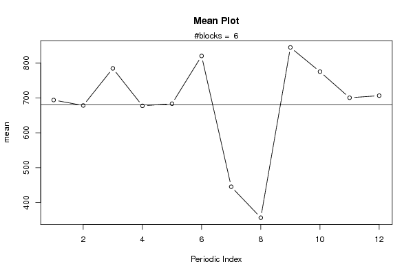
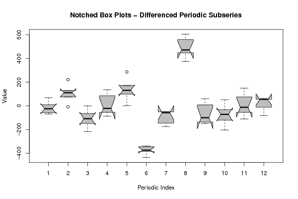
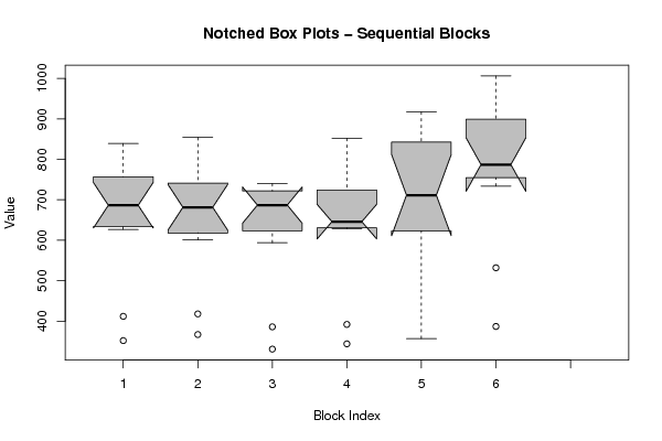
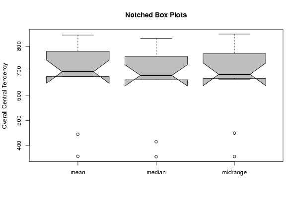
| Title produced by software | Mean Plot | ||||||||||||||||||||
| Date of computation | Fri, 10 Dec 2010 12:05:13 +0000 | ||||||||||||||||||||
| Cite this page as follows | Statistical Computations at FreeStatistics.org, Office for Research Development and Education, URL https://freestatistics.org/blog/index.php?v=date/2010/Dec/10/t1291982860jqhfnlq6a615kns.htm/, Retrieved Mon, 29 Apr 2024 14:41:34 +0000 | ||||||||||||||||||||
| Statistical Computations at FreeStatistics.org, Office for Research Development and Education, URL https://freestatistics.org/blog/index.php?pk=107588, Retrieved Mon, 29 Apr 2024 14:41:34 +0000 | |||||||||||||||||||||
| QR Codes: | |||||||||||||||||||||
|
| |||||||||||||||||||||
| Original text written by user: | |||||||||||||||||||||
| IsPrivate? | No (this computation is public) | ||||||||||||||||||||
| User-defined keywords | |||||||||||||||||||||
| Estimated Impact | 142 | ||||||||||||||||||||
Tree of Dependent Computations | |||||||||||||||||||||
| Family? (F = Feedback message, R = changed R code, M = changed R Module, P = changed Parameters, D = changed Data) | |||||||||||||||||||||
| - [Box-Cox Linearity Plot] [3/11/2009] [2009-11-02 21:47:57] [b98453cac15ba1066b407e146608df68] - D [Box-Cox Linearity Plot] [WS6 box cox] [2009-11-06 12:23:28] [8b1aef4e7013bd33fbc2a5833375c5f5] - RMPD [Mean Plot] [mean & median paper] [2009-12-13 13:22:54] [8b1aef4e7013bd33fbc2a5833375c5f5] - D [Mean Plot] [paper 3.1] [2010-12-10 12:05:13] [5f761c4a622da19727fd2adf71158b48] [Current] | |||||||||||||||||||||
| Feedback Forum | |||||||||||||||||||||
Post a new message | |||||||||||||||||||||
Dataset | |||||||||||||||||||||
| Dataseries X: | |||||||||||||||||||||
627 696 825 677 656 785 412 352 839 729 696 641 695 638 762 635 721 854 418 367 824 687 601 676 740 691 683 594 729 731 386 331 707 715 657 653 642 643 718 654 632 731 392 344 792 852 649 629 685 617 715 715 629 916 531 357 917 828 708 858 775 785 1006 789 734 906 532 387 991 841 892 782 | |||||||||||||||||||||
Tables (Output of Computation) | |||||||||||||||||||||
| |||||||||||||||||||||
Figures (Output of Computation) | |||||||||||||||||||||
Input Parameters & R Code | |||||||||||||||||||||
| Parameters (Session): | |||||||||||||||||||||
| par1 = 12 ; | |||||||||||||||||||||
| Parameters (R input): | |||||||||||||||||||||
| par1 = 12 ; | |||||||||||||||||||||
| R code (references can be found in the software module): | |||||||||||||||||||||
par1 <- as.numeric(par1) | |||||||||||||||||||||