Free Statistics
of Irreproducible Research!
Description of Statistical Computation | |||||||||||||||||||||||||||||||||||||||||||||||||||||||||||||||||
|---|---|---|---|---|---|---|---|---|---|---|---|---|---|---|---|---|---|---|---|---|---|---|---|---|---|---|---|---|---|---|---|---|---|---|---|---|---|---|---|---|---|---|---|---|---|---|---|---|---|---|---|---|---|---|---|---|---|---|---|---|---|---|---|---|---|
| Author's title | |||||||||||||||||||||||||||||||||||||||||||||||||||||||||||||||||
| Author | *The author of this computation has been verified* | ||||||||||||||||||||||||||||||||||||||||||||||||||||||||||||||||
| R Software Module | rwasp_edabi.wasp | ||||||||||||||||||||||||||||||||||||||||||||||||||||||||||||||||
| Title produced by software | Bivariate Explorative Data Analysis | ||||||||||||||||||||||||||||||||||||||||||||||||||||||||||||||||
| Date of computation | Thu, 09 Dec 2010 15:48:00 +0000 | ||||||||||||||||||||||||||||||||||||||||||||||||||||||||||||||||
| Cite this page as follows | Statistical Computations at FreeStatistics.org, Office for Research Development and Education, URL https://freestatistics.org/blog/index.php?v=date/2010/Dec/09/t1291909575rjdc4cwsc92paq2.htm/, Retrieved Mon, 29 Apr 2024 03:23:36 +0000 | ||||||||||||||||||||||||||||||||||||||||||||||||||||||||||||||||
| Statistical Computations at FreeStatistics.org, Office for Research Development and Education, URL https://freestatistics.org/blog/index.php?pk=107228, Retrieved Mon, 29 Apr 2024 03:23:36 +0000 | |||||||||||||||||||||||||||||||||||||||||||||||||||||||||||||||||
| QR Codes: | |||||||||||||||||||||||||||||||||||||||||||||||||||||||||||||||||
|
| |||||||||||||||||||||||||||||||||||||||||||||||||||||||||||||||||
| Original text written by user: | |||||||||||||||||||||||||||||||||||||||||||||||||||||||||||||||||
| IsPrivate? | No (this computation is public) | ||||||||||||||||||||||||||||||||||||||||||||||||||||||||||||||||
| User-defined keywords | Paper dma | ||||||||||||||||||||||||||||||||||||||||||||||||||||||||||||||||
| Estimated Impact | 203 | ||||||||||||||||||||||||||||||||||||||||||||||||||||||||||||||||
Tree of Dependent Computations | |||||||||||||||||||||||||||||||||||||||||||||||||||||||||||||||||
| Family? (F = Feedback message, R = changed R code, M = changed R Module, P = changed Parameters, D = changed Data) | |||||||||||||||||||||||||||||||||||||||||||||||||||||||||||||||||
| - [Bivariate Data Series] [Bivariate dataset] [2008-01-05 23:51:08] [74be16979710d4c4e7c6647856088456] - RMPD [Bivariate Explorative Data Analysis] [Ws4 part 1.1 s090...] [2009-10-27 21:56:53] [e0fc65a5811681d807296d590d5b45de] - M D [Bivariate Explorative Data Analysis] [Paper; bivariate ...] [2009-12-19 19:10:37] [e0fc65a5811681d807296d590d5b45de] - RMPD [] [PAPER DMA Bivaria...] [-0001-11-30 00:00:00] [74be16979710d4c4e7c6647856088456] - RMPD [Bivariate Explorative Data Analysis] [Biveriate EDA Pap...] [2010-12-09 15:48:00] [f92ba2b01007f169e2985fcc57236bd0] [Current] - D [Bivariate Explorative Data Analysis] [] [2010-12-13 09:53:42] [1251ac2db27b84d4a3ba43449388906b] - [Bivariate Explorative Data Analysis] [workshop 10: Mult...] [2010-12-14 08:27:59] [814f53995537cd15c528d8efbf1cf544] | |||||||||||||||||||||||||||||||||||||||||||||||||||||||||||||||||
| Feedback Forum | |||||||||||||||||||||||||||||||||||||||||||||||||||||||||||||||||
Post a new message | |||||||||||||||||||||||||||||||||||||||||||||||||||||||||||||||||
Dataset | |||||||||||||||||||||||||||||||||||||||||||||||||||||||||||||||||
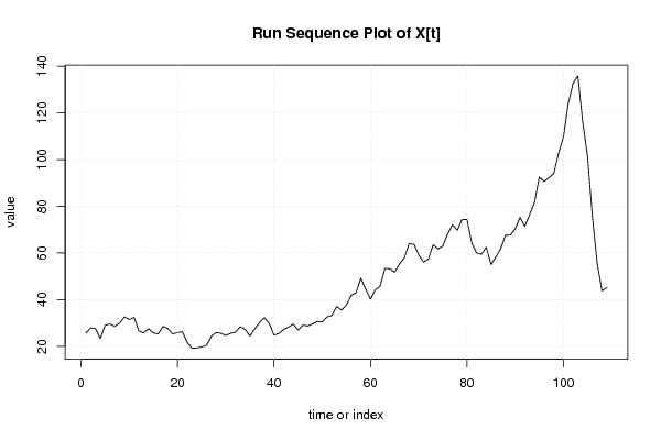
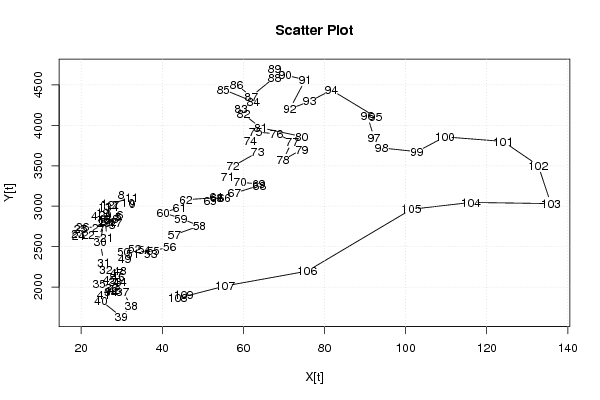
| Dataseries X: | |||||||||||||||||||||||||||||||||||||||||||||||||||||||||||||||||
25.64 27.97 27.62 23.31 29.07 29.58 28.63 29.92 32.68 31.54 32.43 26.54 25.85 27.6 25.71 25.38 28.57 27.64 25.36 25.9 26.29 21.74 19.2 19.32 19.82 20.36 24.31 25.97 25.61 24.67 25.59 26.09 28.37 27.34 24.46 27.46 30.23 32.33 29.87 24.87 25.48 27.28 28.24 29.58 26.95 29.08 28.76 29.59 30.7 30.52 32.67 33.19 37.13 35.54 37.75 41.84 42.94 49.14 44.61 40.22 44.23 45.85 53.38 53.26 51.8 55.3 57.81 63.96 63.77 59.15 56.12 57.42 63.52 61.71 63.01 68.18 72.03 69.75 74.41 74.33 64.24 60.03 59.44 62.5 55.04 58.34 61.92 67.65 67.68 70.3 75.26 71.44 76.36 81.71 92.6 90.6 92.23 94.09 102.79 109.65 124.05 132.69 135.81 116.07 101.42 75.73 55.48 43.8 45.29 | |||||||||||||||||||||||||||||||||||||||||||||||||||||||||||||||||
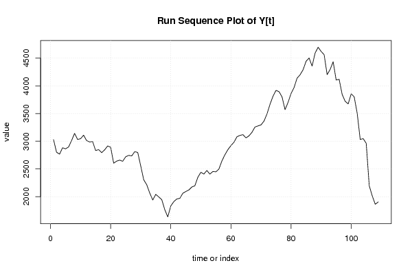
| Dataseries Y: | |||||||||||||||||||||||||||||||||||||||||||||||||||||||||||||||||
3030,29 2803,47 2767,63 2882,6 2863,36 2897,06 3012,61 3142,95 3032,93 3045,78 3110,52 3013,24 2987,1 2995,55 2833,18 2848,96 2794,83 2845,26 2915,03 2892,63 2604,42 2641,65 2659,81 2638,53 2720,25 2745,88 2735,7 2811,7 2799,43 2555,28 2304,98 2214,95 2065,81 1940,49 2042 1995,37 1946,81 1765,9 1635,25 1833,42 1910,43 1959,67 1969,6 2061,41 2093,48 2120,88 2174,56 2196,72 2350,44 2440,25 2408,64 2472,81 2407,6 2454,62 2448,05 2497,84 2645,64 2756,76 2849,27 2921,44 2981,85 3080,58 3106,22 3119,31 3061,26 3097,31 3161,69 3257,16 3277,01 3295,32 3363,99 3494,17 3667,03 3813,06 3917,96 3895,51 3801,06 3570,12 3701,61 3862,27 3970,1 4138,52 4199,75 4290,89 4443,91 4502,64 4356,98 4591,27 4696,96 4621,4 4562,84 4202,52 4296,49 4435,23 4105,18 4116,68 3844,49 3720,98 3674,4 3857,62 3801,06 3504,37 3032,6 3047,03 2962,34 2197,82 2014,45 1862,83 1905,41 | |||||||||||||||||||||||||||||||||||||||||||||||||||||||||||||||||
Tables (Output of Computation) | |||||||||||||||||||||||||||||||||||||||||||||||||||||||||||||||||
| |||||||||||||||||||||||||||||||||||||||||||||||||||||||||||||||||
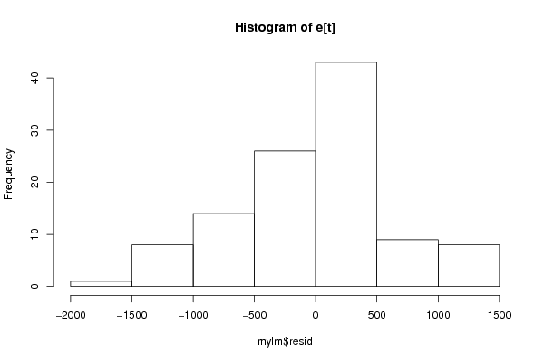
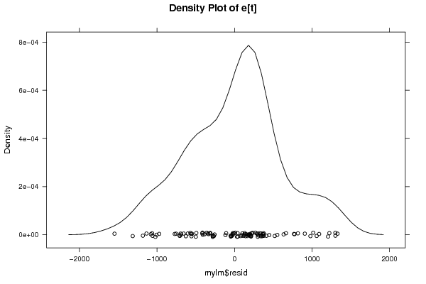
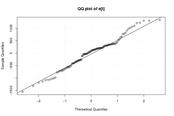
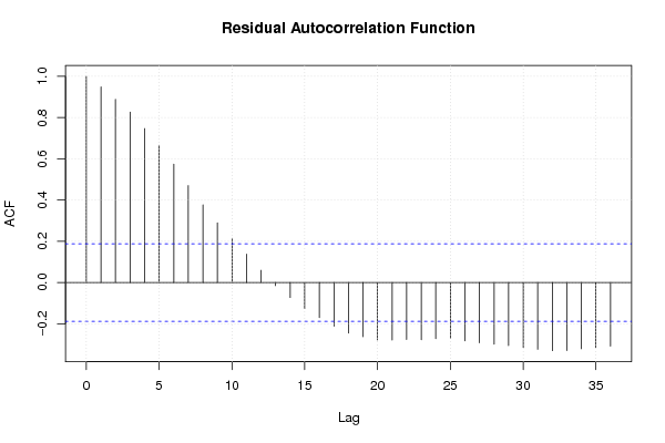
Figures (Output of Computation) | |||||||||||||||||||||||||||||||||||||||||||||||||||||||||||||||||
Input Parameters & R Code | |||||||||||||||||||||||||||||||||||||||||||||||||||||||||||||||||
| Parameters (Session): | |||||||||||||||||||||||||||||||||||||||||||||||||||||||||||||||||
| par1 = 0 ; par2 = 36 ; | |||||||||||||||||||||||||||||||||||||||||||||||||||||||||||||||||
| Parameters (R input): | |||||||||||||||||||||||||||||||||||||||||||||||||||||||||||||||||
| par1 = 0 ; par2 = 36 ; | |||||||||||||||||||||||||||||||||||||||||||||||||||||||||||||||||
| R code (references can be found in the software module): | |||||||||||||||||||||||||||||||||||||||||||||||||||||||||||||||||
par1 <- as.numeric(par1) | |||||||||||||||||||||||||||||||||||||||||||||||||||||||||||||||||