Free Statistics
of Irreproducible Research!
Description of Statistical Computation | |||||||||||||||||||||||||||||||||||||||||||||||||||||
|---|---|---|---|---|---|---|---|---|---|---|---|---|---|---|---|---|---|---|---|---|---|---|---|---|---|---|---|---|---|---|---|---|---|---|---|---|---|---|---|---|---|---|---|---|---|---|---|---|---|---|---|---|---|
| Author's title | |||||||||||||||||||||||||||||||||||||||||||||||||||||
| Author | *The author of this computation has been verified* | ||||||||||||||||||||||||||||||||||||||||||||||||||||
| R Software Module | rwasp_edauni.wasp | ||||||||||||||||||||||||||||||||||||||||||||||||||||
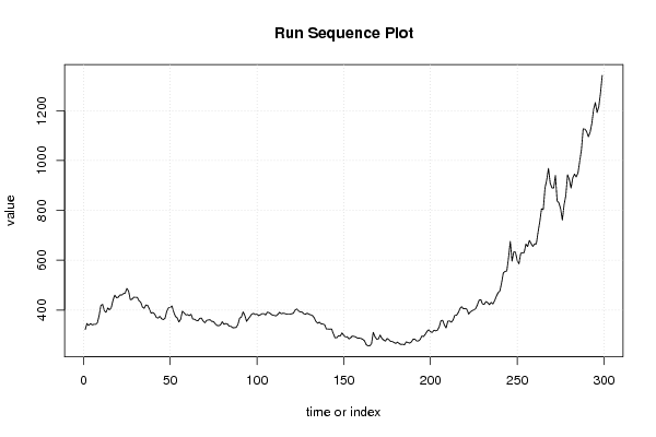
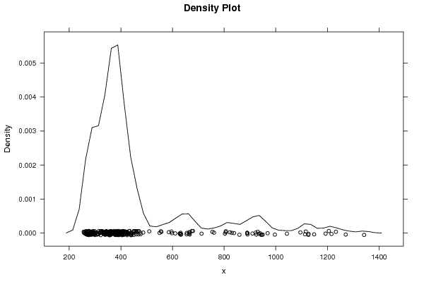
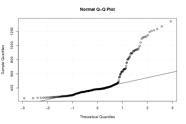
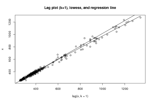
| Title produced by software | Univariate Explorative Data Analysis | ||||||||||||||||||||||||||||||||||||||||||||||||||||
| Date of computation | Tue, 07 Dec 2010 21:00:08 +0000 | ||||||||||||||||||||||||||||||||||||||||||||||||||||
| Cite this page as follows | Statistical Computations at FreeStatistics.org, Office for Research Development and Education, URL https://freestatistics.org/blog/index.php?v=date/2010/Dec/07/t1291755504h6tjy99m2lhfyxj.htm/, Retrieved Fri, 03 May 2024 23:59:01 +0000 | ||||||||||||||||||||||||||||||||||||||||||||||||||||
| Statistical Computations at FreeStatistics.org, Office for Research Development and Education, URL https://freestatistics.org/blog/index.php?pk=106739, Retrieved Fri, 03 May 2024 23:59:01 +0000 | |||||||||||||||||||||||||||||||||||||||||||||||||||||
| QR Codes: | |||||||||||||||||||||||||||||||||||||||||||||||||||||
|
| |||||||||||||||||||||||||||||||||||||||||||||||||||||
| Original text written by user: | |||||||||||||||||||||||||||||||||||||||||||||||||||||
| IsPrivate? | No (this computation is public) | ||||||||||||||||||||||||||||||||||||||||||||||||||||
| User-defined keywords | |||||||||||||||||||||||||||||||||||||||||||||||||||||
| Estimated Impact | 141 | ||||||||||||||||||||||||||||||||||||||||||||||||||||
Tree of Dependent Computations | |||||||||||||||||||||||||||||||||||||||||||||||||||||
| Family? (F = Feedback message, R = changed R code, M = changed R Module, P = changed Parameters, D = changed Data) | |||||||||||||||||||||||||||||||||||||||||||||||||||||
| - [Univariate Explorative Data Analysis] [time effect in su...] [2010-11-17 08:55:33] [b98453cac15ba1066b407e146608df68] - R D [Univariate Explorative Data Analysis] [WS7 Tutorial Popu...] [2010-11-22 10:43:52] [afe9379cca749d06b3d6872e02cc47ed] - [Univariate Explorative Data Analysis] [WS 4: Run Sequenc...] [2010-12-02 17:30:51] [4f1a20f787b3465111b61213cdeef1a9] - D [Univariate Explorative Data Analysis] [WS 4: Run Sequenc...] [2010-12-07 21:00:08] [f0b33ae54e73edcd25a3e2f31270d1c9] [Current] | |||||||||||||||||||||||||||||||||||||||||||||||||||||
| Feedback Forum | |||||||||||||||||||||||||||||||||||||||||||||||||||||
Post a new message | |||||||||||||||||||||||||||||||||||||||||||||||||||||
Dataset | |||||||||||||||||||||||||||||||||||||||||||||||||||||
| Dataseries X: | |||||||||||||||||||||||||||||||||||||||||||||||||||||
321.61 345.85 338.60 345.64 340.71 342.49 342.65 348.68 377.36 418.05 423.13 397.69 390.80 408.29 401.02 409.24 439.28 459.95 449.66 451.14 460.66 460.23 465.69 468.01 486.74 475.89 441.52 443.63 451.62 451.14 450.88 437.56 431.18 412.02 407.14 420.48 418.92 403.57 387.55 390.02 384.37 370.62 367.90 374.91 365.15 361.91 367.03 395.19 409.25 410.49 416.58 392.21 374.29 369.05 352.19 362.85 395.47 388.82 380.39 381.73 377.69 383.04 363.89 363.23 358.37 356.97 366.87 367.57 355.88 348.88 358.77 360.42 361.08 354.57 353.73 344.20 338.34 337.21 340.96 353.29 342.67 345.71 344.17 334.92 334.81 329.05 329.31 330.25 341.89 367.74 371.93 392.79 377.97 354.93 364.40 374.05 383.63 386.56 381.90 384.08 377.29 381.54 385.60 385.47 380.40 391.74 389.57 384.29 379.26 378.44 376.63 382.48 390.89 385.04 387.58 386.19 383.78 383.10 383.25 385.19 387.35 400.49 404.53 396.15 392.79 391.96 385.04 383.58 387.46 382.90 381.04 377.69 368.95 353.87 347.03 351.49 344.23 344.09 340.51 323.90 324.02 323.11 324.36 305.55 288.59 289.15 297.49 295.94 308.29 299.10 292.32 292.87 284.11 288.98 295.93 294.17 291.68 287.07 287.33 285.96 282.62 276.44 261.31 256.08 256.69 264.74 310.72 293.18 283.07 284.32 299.86 286.39 279.69 275.19 285.73 281.59 274.47 273.68 270.00 266.01 271.45 265.49 261.87 263.03 260.48 272.36 269.82 267.53 272.39 283.42 283.06 276.16 275.85 281.51 295.50 294.06 302.68 314.58 321.18 313.29 310.25 319.14 316.56 319.07 331.92 356.86 358.97 340.55 328.18 355.68 356.35 350.99 359.77 378.95 378.92 389.91 406.11 413.79 404.95 406.67 403.26 383.78 392.48 398.09 400.51 405.28 420.46 439.38 442.08 424.03 423.35 434.32 429.23 421.87 430.66 424.48 437.93 456.05 469.90 476.67 510.10 549.86 555.00 557.09 610.65 675.39 596.15 633.71 632.33 598.06 585.78 627.83 629.42 631.17 664.75 654.90 679.37 666.92 655.49 665.30 665.41 712.65 754.60 806.25 803.20 889.60 922.30 968.43 909.70 890.51 889.49 939.77 838.31 829.93 806.62 760.86 822.00 859.19 943.16 924.27 889.50 930.20 945.67 934.23 949.67 996.59 1043.16 1127.04 1126.22 1116.51 1095.41 1113.34 1148.69 1205.43 1232.92 1192.97 1215.81 1270.98 1342.02 | |||||||||||||||||||||||||||||||||||||||||||||||||||||
Tables (Output of Computation) | |||||||||||||||||||||||||||||||||||||||||||||||||||||
| |||||||||||||||||||||||||||||||||||||||||||||||||||||
Figures (Output of Computation) | |||||||||||||||||||||||||||||||||||||||||||||||||||||
Input Parameters & R Code | |||||||||||||||||||||||||||||||||||||||||||||||||||||
| Parameters (Session): | |||||||||||||||||||||||||||||||||||||||||||||||||||||
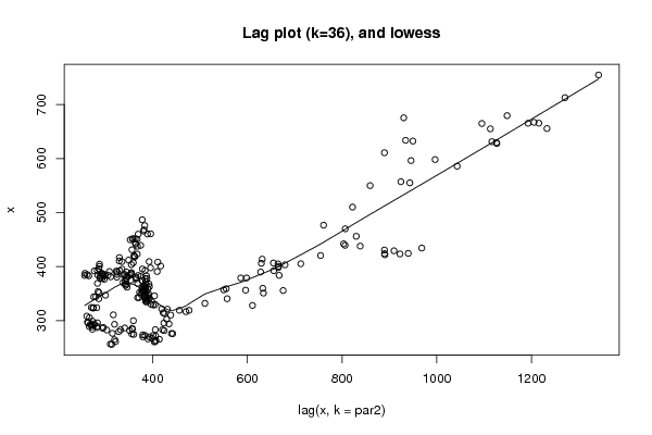
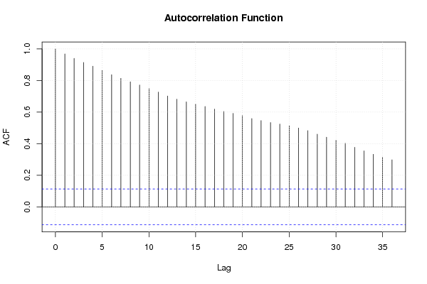
| par1 = 0 ; par2 = 36 ; | |||||||||||||||||||||||||||||||||||||||||||||||||||||
| Parameters (R input): | |||||||||||||||||||||||||||||||||||||||||||||||||||||
| par1 = 0 ; par2 = 36 ; | |||||||||||||||||||||||||||||||||||||||||||||||||||||
| R code (references can be found in the software module): | |||||||||||||||||||||||||||||||||||||||||||||||||||||
par1 <- as.numeric(par1) | |||||||||||||||||||||||||||||||||||||||||||||||||||||