Repository of Reproducible Computations

Free Statistics

of Irreproducible Research!

Author's title

Author

*The author of this computation has been verified*

R Software Module

rwasp_autocorrelation.wasp

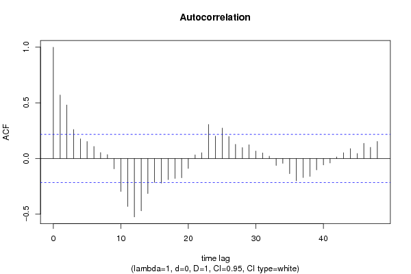
Title produced by software

(Partial) Autocorrelation Function

Date of computation

Tue, 07 Dec 2010 15:46:19 +0000

Cite this page as follows

Statistical Computations at FreeStatistics.org, Office for Research Development and Education, URL https://freestatistics.org/blog/index.php?v=date/2010/Dec/07/t129173666813lh9oy9zf8v4zj.htm/, Retrieved Fri, 03 May 2024 18:34:24 +0000

Statistical Computations at FreeStatistics.org, Office for Research Development and Education, URL https://freestatistics.org/blog/index.php?pk=106446, Retrieved Fri, 03 May 2024 18:34:24 +0000

QR Codes:

Paste this QR Code to cite your computation.

Original text written by user:

IsPrivate?

No (this computation is public)

User-defined keywords

Estimated Impact

164

Family? (F = Feedback message, R = changed R code, M = changed R Module, P = changed Parameters, D = changed Data)

-     [Univariate Data Series] [data set] [2008-12-01 19:54:57] [b98453cac15ba1066b407e146608df68]
- RMP   [(Partial) Autocorrelation Function] [Unemployment] [2010-11-29 09:05:21] [b98453cac15ba1066b407e146608df68]
-   PD    [(Partial) Autocorrelation Function] [ACF geen differen...] [2010-12-03 12:24:26] [9f32078fdcdc094ca748857d5ebdb3de]
-    D      [(Partial) Autocorrelation Function] [] [2010-12-07 15:41:58] [ed939ef6f97e5f2afb6796311d9e7a5f]
-   P           [(Partial) Autocorrelation Function] [] [2010-12-07 15:46:19] [f9aa24c2294a5d3925c7278aa2e9a372] [Current]
- R PD            [(Partial) Autocorrelation Function] [ACF d=1, D=1] [2010-12-08 16:49:09] [1f5baf2b24e732d76900bb8178fc04e7] 

Feedback Forum

Post a new message

Dataseries X:

Download CSV

Histogram

Boxplots

Summary of computational transaction
Raw Input	view raw input (R code)
Raw Output	view raw output of R engine
Computing time	2 seconds
R Server	'RServer@AstonUniversity' @ vre.aston.ac.uk

\begin{tabular}{lllllllll}
\hline
Summary of computational transaction \tabularnewline
Raw Input & view raw input (R code)  \tabularnewline
Raw Output & view raw output of R engine  \tabularnewline
Computing time & 2 seconds \tabularnewline
R Server & 'RServer@AstonUniversity' @ vre.aston.ac.uk \tabularnewline
\hline
\end{tabular}
%Source: https://freestatistics.org/blog/index.php?pk=106446&T=0

[TABLE]
[ROW][C]Summary of computational transaction[/C][/ROW]
[ROW][C]Raw Input[/C][C]view raw input (R code) [/C][/ROW]
[ROW][C]Raw Output[/C][C]view raw output of R engine [/C][/ROW]
[ROW][C]Computing time[/C][C]2 seconds[/C][/ROW]
[ROW][C]R Server[/C][C]'RServer@AstonUniversity' @ vre.aston.ac.uk[/C][/ROW]
[/TABLE]
Source: https://freestatistics.org/blog/index.php?pk=106446&T=0

Globally Unique Identifier (entire table): ba.freestatistics.org/blog/index.php?pk=106446&T=0

As an alternative you can also use a QR Code:

The GUIDs for individual cells are displayed in the table below:

Summary of computational transaction
Raw Input	view raw input (R code)
Raw Output	view raw output of R engine
Computing time	2 seconds
R Server	'RServer@AstonUniversity' @ vre.aston.ac.uk

Autocorrelation Function
Time lag k	ACF(k)	T-STAT	P-value
1	0.570108	5.1625	1e-06
2	0.480446	4.3506	1.9e-05
3	0.260015	2.3545	0.010468
4	0.175678	1.5908	0.057748
5	0.152204	1.3783	0.085936
6	0.107526	0.9737	0.166536
7	0.05342	0.4837	0.314932
8	0.034165	0.3094	0.37891
9	-0.093307	-0.8449	0.200304
10	-0.296493	-2.6849	0.004389
11	-0.431528	-3.9077	9.5e-05
12	-0.525495	-4.7586	4e-06
13	-0.47135	-4.2683	2.6e-05
14	-0.314983	-2.8523	0.002746
15	-0.215803	-1.9542	0.027044
16	-0.221377	-2.0047	0.02415
17	-0.189834	-1.719	0.044692
18	-0.179489	-1.6253	0.053964
19	-0.174073	-1.5763	0.059404
20	-0.0899	-0.8141	0.208978
21	0.03231	0.2926	0.385291
22	0.051806	0.4691	0.320112
23	0.305935	2.7704	0.003462
24	0.200151	1.8124	0.036788
25	0.273551	2.4771	0.00765
26	0.196991	1.7838	0.039076
27	0.12633	1.144	0.127982
28	0.097931	0.8868	0.188888
29	0.123046	1.1142	0.134218
30	0.066301	0.6004	0.274955
31	0.049895	0.4518	0.326295
32	0.020677	0.1872	0.425968
33	-0.062372	-0.5648	0.286874
34	-0.043776	-0.3964	0.346417
35	-0.136853	-1.2393	0.109393
36	-0.201056	-1.8206	0.036155
37	-0.17132	-1.5514	0.062333
38	-0.161384	-1.4614	0.073865
39	-0.102567	-0.9288	0.177863
40	-0.058208	-0.5271	0.299776
41	-0.040701	-0.3686	0.356701
42	0.013784	0.1248	0.450485
43	0.05171	0.4683	0.320421
44	0.087996	0.7968	0.213923
45	0.044546	0.4034	0.34386
46	0.136555	1.2366	0.109891
47	0.100111	0.9065	0.183652
48	0.153298	1.3882	0.084422

\begin{tabular}{lllllllll}
\hline
Autocorrelation Function \tabularnewline
Time lag k & ACF(k) & T-STAT & P-value \tabularnewline
1 & 0.570108 & 5.1625 & 1e-06 \tabularnewline
2 & 0.480446 & 4.3506 & 1.9e-05 \tabularnewline
3 & 0.260015 & 2.3545 & 0.010468 \tabularnewline
4 & 0.175678 & 1.5908 & 0.057748 \tabularnewline
5 & 0.152204 & 1.3783 & 0.085936 \tabularnewline
6 & 0.107526 & 0.9737 & 0.166536 \tabularnewline
7 & 0.05342 & 0.4837 & 0.314932 \tabularnewline
8 & 0.034165 & 0.3094 & 0.37891 \tabularnewline
9 & -0.093307 & -0.8449 & 0.200304 \tabularnewline
10 & -0.296493 & -2.6849 & 0.004389 \tabularnewline
11 & -0.431528 & -3.9077 & 9.5e-05 \tabularnewline
12 & -0.525495 & -4.7586 & 4e-06 \tabularnewline
13 & -0.47135 & -4.2683 & 2.6e-05 \tabularnewline
14 & -0.314983 & -2.8523 & 0.002746 \tabularnewline
15 & -0.215803 & -1.9542 & 0.027044 \tabularnewline
16 & -0.221377 & -2.0047 & 0.02415 \tabularnewline
17 & -0.189834 & -1.719 & 0.044692 \tabularnewline
18 & -0.179489 & -1.6253 & 0.053964 \tabularnewline
19 & -0.174073 & -1.5763 & 0.059404 \tabularnewline
20 & -0.0899 & -0.8141 & 0.208978 \tabularnewline
21 & 0.03231 & 0.2926 & 0.385291 \tabularnewline
22 & 0.051806 & 0.4691 & 0.320112 \tabularnewline
23 & 0.305935 & 2.7704 & 0.003462 \tabularnewline
24 & 0.200151 & 1.8124 & 0.036788 \tabularnewline
25 & 0.273551 & 2.4771 & 0.00765 \tabularnewline
26 & 0.196991 & 1.7838 & 0.039076 \tabularnewline
27 & 0.12633 & 1.144 & 0.127982 \tabularnewline
28 & 0.097931 & 0.8868 & 0.188888 \tabularnewline
29 & 0.123046 & 1.1142 & 0.134218 \tabularnewline
30 & 0.066301 & 0.6004 & 0.274955 \tabularnewline
31 & 0.049895 & 0.4518 & 0.326295 \tabularnewline
32 & 0.020677 & 0.1872 & 0.425968 \tabularnewline
33 & -0.062372 & -0.5648 & 0.286874 \tabularnewline
34 & -0.043776 & -0.3964 & 0.346417 \tabularnewline
35 & -0.136853 & -1.2393 & 0.109393 \tabularnewline
36 & -0.201056 & -1.8206 & 0.036155 \tabularnewline
37 & -0.17132 & -1.5514 & 0.062333 \tabularnewline
38 & -0.161384 & -1.4614 & 0.073865 \tabularnewline
39 & -0.102567 & -0.9288 & 0.177863 \tabularnewline
40 & -0.058208 & -0.5271 & 0.299776 \tabularnewline
41 & -0.040701 & -0.3686 & 0.356701 \tabularnewline
42 & 0.013784 & 0.1248 & 0.450485 \tabularnewline
43 & 0.05171 & 0.4683 & 0.320421 \tabularnewline
44 & 0.087996 & 0.7968 & 0.213923 \tabularnewline
45 & 0.044546 & 0.4034 & 0.34386 \tabularnewline
46 & 0.136555 & 1.2366 & 0.109891 \tabularnewline
47 & 0.100111 & 0.9065 & 0.183652 \tabularnewline
48 & 0.153298 & 1.3882 & 0.084422 \tabularnewline
\hline
\end{tabular}
%Source: https://freestatistics.org/blog/index.php?pk=106446&T=1

[TABLE]
[ROW][C]Autocorrelation Function[/C][/ROW]
[ROW][C]Time lag k[/C][C]ACF(k)[/C][C]T-STAT[/C][C]P-value[/C][/ROW]
[ROW][C]1[/C][C]0.570108[/C][C]5.1625[/C][C]1e-06[/C][/ROW]
[ROW][C]2[/C][C]0.480446[/C][C]4.3506[/C][C]1.9e-05[/C][/ROW]
[ROW][C]3[/C][C]0.260015[/C][C]2.3545[/C][C]0.010468[/C][/ROW]
[ROW][C]4[/C][C]0.175678[/C][C]1.5908[/C][C]0.057748[/C][/ROW]
[ROW][C]5[/C][C]0.152204[/C][C]1.3783[/C][C]0.085936[/C][/ROW]
[ROW][C]6[/C][C]0.107526[/C][C]0.9737[/C][C]0.166536[/C][/ROW]
[ROW][C]7[/C][C]0.05342[/C][C]0.4837[/C][C]0.314932[/C][/ROW]
[ROW][C]8[/C][C]0.034165[/C][C]0.3094[/C][C]0.37891[/C][/ROW]
[ROW][C]9[/C][C]-0.093307[/C][C]-0.8449[/C][C]0.200304[/C][/ROW]
[ROW][C]10[/C][C]-0.296493[/C][C]-2.6849[/C][C]0.004389[/C][/ROW]
[ROW][C]11[/C][C]-0.431528[/C][C]-3.9077[/C][C]9.5e-05[/C][/ROW]
[ROW][C]12[/C][C]-0.525495[/C][C]-4.7586[/C][C]4e-06[/C][/ROW]
[ROW][C]13[/C][C]-0.47135[/C][C]-4.2683[/C][C]2.6e-05[/C][/ROW]
[ROW][C]14[/C][C]-0.314983[/C][C]-2.8523[/C][C]0.002746[/C][/ROW]
[ROW][C]15[/C][C]-0.215803[/C][C]-1.9542[/C][C]0.027044[/C][/ROW]
[ROW][C]16[/C][C]-0.221377[/C][C]-2.0047[/C][C]0.02415[/C][/ROW]
[ROW][C]17[/C][C]-0.189834[/C][C]-1.719[/C][C]0.044692[/C][/ROW]
[ROW][C]18[/C][C]-0.179489[/C][C]-1.6253[/C][C]0.053964[/C][/ROW]
[ROW][C]19[/C][C]-0.174073[/C][C]-1.5763[/C][C]0.059404[/C][/ROW]
[ROW][C]20[/C][C]-0.0899[/C][C]-0.8141[/C][C]0.208978[/C][/ROW]
[ROW][C]21[/C][C]0.03231[/C][C]0.2926[/C][C]0.385291[/C][/ROW]
[ROW][C]22[/C][C]0.051806[/C][C]0.4691[/C][C]0.320112[/C][/ROW]
[ROW][C]23[/C][C]0.305935[/C][C]2.7704[/C][C]0.003462[/C][/ROW]
[ROW][C]24[/C][C]0.200151[/C][C]1.8124[/C][C]0.036788[/C][/ROW]
[ROW][C]25[/C][C]0.273551[/C][C]2.4771[/C][C]0.00765[/C][/ROW]
[ROW][C]26[/C][C]0.196991[/C][C]1.7838[/C][C]0.039076[/C][/ROW]
[ROW][C]27[/C][C]0.12633[/C][C]1.144[/C][C]0.127982[/C][/ROW]
[ROW][C]28[/C][C]0.097931[/C][C]0.8868[/C][C]0.188888[/C][/ROW]
[ROW][C]29[/C][C]0.123046[/C][C]1.1142[/C][C]0.134218[/C][/ROW]
[ROW][C]30[/C][C]0.066301[/C][C]0.6004[/C][C]0.274955[/C][/ROW]
[ROW][C]31[/C][C]0.049895[/C][C]0.4518[/C][C]0.326295[/C][/ROW]
[ROW][C]32[/C][C]0.020677[/C][C]0.1872[/C][C]0.425968[/C][/ROW]
[ROW][C]33[/C][C]-0.062372[/C][C]-0.5648[/C][C]0.286874[/C][/ROW]
[ROW][C]34[/C][C]-0.043776[/C][C]-0.3964[/C][C]0.346417[/C][/ROW]
[ROW][C]35[/C][C]-0.136853[/C][C]-1.2393[/C][C]0.109393[/C][/ROW]
[ROW][C]36[/C][C]-0.201056[/C][C]-1.8206[/C][C]0.036155[/C][/ROW]
[ROW][C]37[/C][C]-0.17132[/C][C]-1.5514[/C][C]0.062333[/C][/ROW]
[ROW][C]38[/C][C]-0.161384[/C][C]-1.4614[/C][C]0.073865[/C][/ROW]
[ROW][C]39[/C][C]-0.102567[/C][C]-0.9288[/C][C]0.177863[/C][/ROW]
[ROW][C]40[/C][C]-0.058208[/C][C]-0.5271[/C][C]0.299776[/C][/ROW]
[ROW][C]41[/C][C]-0.040701[/C][C]-0.3686[/C][C]0.356701[/C][/ROW]
[ROW][C]42[/C][C]0.013784[/C][C]0.1248[/C][C]0.450485[/C][/ROW]
[ROW][C]43[/C][C]0.05171[/C][C]0.4683[/C][C]0.320421[/C][/ROW]
[ROW][C]44[/C][C]0.087996[/C][C]0.7968[/C][C]0.213923[/C][/ROW]
[ROW][C]45[/C][C]0.044546[/C][C]0.4034[/C][C]0.34386[/C][/ROW]
[ROW][C]46[/C][C]0.136555[/C][C]1.2366[/C][C]0.109891[/C][/ROW]
[ROW][C]47[/C][C]0.100111[/C][C]0.9065[/C][C]0.183652[/C][/ROW]
[ROW][C]48[/C][C]0.153298[/C][C]1.3882[/C][C]0.084422[/C][/ROW]
[/TABLE]
Source: https://freestatistics.org/blog/index.php?pk=106446&T=1

Globally Unique Identifier (entire table): ba.freestatistics.org/blog/index.php?pk=106446&T=1

As an alternative you can also use a QR Code:

The GUIDs for individual cells are displayed in the table below:

Autocorrelation Function
Time lag k	ACF(k)	T-STAT	P-value
1	0.570108	5.1625	1e-06
2	0.480446	4.3506	1.9e-05
3	0.260015	2.3545	0.010468
4	0.175678	1.5908	0.057748
5	0.152204	1.3783	0.085936
6	0.107526	0.9737	0.166536
7	0.05342	0.4837	0.314932
8	0.034165	0.3094	0.37891
9	-0.093307	-0.8449	0.200304
10	-0.296493	-2.6849	0.004389
11	-0.431528	-3.9077	9.5e-05
12	-0.525495	-4.7586	4e-06
13	-0.47135	-4.2683	2.6e-05
14	-0.314983	-2.8523	0.002746
15	-0.215803	-1.9542	0.027044
16	-0.221377	-2.0047	0.02415
17	-0.189834	-1.719	0.044692
18	-0.179489	-1.6253	0.053964
19	-0.174073	-1.5763	0.059404
20	-0.0899	-0.8141	0.208978
21	0.03231	0.2926	0.385291
22	0.051806	0.4691	0.320112
23	0.305935	2.7704	0.003462
24	0.200151	1.8124	0.036788
25	0.273551	2.4771	0.00765
26	0.196991	1.7838	0.039076
27	0.12633	1.144	0.127982
28	0.097931	0.8868	0.188888
29	0.123046	1.1142	0.134218
30	0.066301	0.6004	0.274955
31	0.049895	0.4518	0.326295
32	0.020677	0.1872	0.425968
33	-0.062372	-0.5648	0.286874
34	-0.043776	-0.3964	0.346417
35	-0.136853	-1.2393	0.109393
36	-0.201056	-1.8206	0.036155
37	-0.17132	-1.5514	0.062333
38	-0.161384	-1.4614	0.073865
39	-0.102567	-0.9288	0.177863
40	-0.058208	-0.5271	0.299776
41	-0.040701	-0.3686	0.356701
42	0.013784	0.1248	0.450485
43	0.05171	0.4683	0.320421
44	0.087996	0.7968	0.213923
45	0.044546	0.4034	0.34386
46	0.136555	1.2366	0.109891
47	0.100111	0.9065	0.183652
48	0.153298	1.3882	0.084422

Partial Autocorrelation Function
Time lag k	PACF(k)	T-STAT	P-value
1	0.570108	5.1625	1e-06
2	0.230264	2.0851	0.020084
3	-0.128437	-1.163	0.124091
4	-0.016863	-0.1527	0.439504
5	0.098712	0.8939	0.187002
6	-0.006787	-0.0615	0.47557
7	-0.073805	-0.6683	0.252899
8	0.013561	0.1228	0.451282
9	-0.154849	-1.4022	0.082312
10	-0.349734	-3.167	0.001082
11	-0.23142	-2.0956	0.019601
12	-0.163321	-1.4789	0.071495
13	-0.055184	-0.4997	0.309308
14	0.155317	1.4065	0.081684
15	0.126529	1.1458	0.127612
16	-0.122802	-1.112	0.13469
17	-0.015956	-0.1445	0.442736
18	0.090862	0.8228	0.206506
19	-0.064622	-0.5852	0.280017
20	-0.001559	-0.0141	0.494384
21	0.124238	1.125	0.131932
22	-0.278079	-2.5181	0.006872
23	0.149499	1.3538	0.089765
24	-0.10885	-0.9857	0.163595
25	0.016663	0.1509	0.440217
26	0.054542	0.4939	0.311349
27	-0.052799	-0.4781	0.316919
28	-0.162605	-1.4725	0.072363
29	0.000325	0.0029	0.498828
30	-0.058582	-0.5305	0.298606
31	-0.128363	-1.1624	0.124228
32	0.043468	0.3936	0.34744
33	0.027354	0.2477	0.402491
34	0.043359	0.3926	0.347806
35	-0.016627	-0.1506	0.440346
36	-0.071422	-0.6468	0.259799
37	0.01962	0.1777	0.42971
38	-0.040423	-0.366	0.357637
39	0.078935	0.7148	0.238387
40	-0.008173	-0.074	0.470593
41	-0.051521	-0.4665	0.321033
42	0.128178	1.1607	0.124565
43	0.007359	0.0666	0.473515
44	-0.031927	-0.2891	0.386614
45	0.06311	0.5715	0.284616
46	-0.013119	-0.1188	0.452865
47	-0.085715	-0.7762	0.219938
48	-0.080206	-0.7263	0.234863

\begin{tabular}{lllllllll}
\hline
Partial Autocorrelation Function \tabularnewline
Time lag k & PACF(k) & T-STAT & P-value \tabularnewline
1 & 0.570108 & 5.1625 & 1e-06 \tabularnewline
2 & 0.230264 & 2.0851 & 0.020084 \tabularnewline
3 & -0.128437 & -1.163 & 0.124091 \tabularnewline
4 & -0.016863 & -0.1527 & 0.439504 \tabularnewline
5 & 0.098712 & 0.8939 & 0.187002 \tabularnewline
6 & -0.006787 & -0.0615 & 0.47557 \tabularnewline
7 & -0.073805 & -0.6683 & 0.252899 \tabularnewline
8 & 0.013561 & 0.1228 & 0.451282 \tabularnewline
9 & -0.154849 & -1.4022 & 0.082312 \tabularnewline
10 & -0.349734 & -3.167 & 0.001082 \tabularnewline
11 & -0.23142 & -2.0956 & 0.019601 \tabularnewline
12 & -0.163321 & -1.4789 & 0.071495 \tabularnewline
13 & -0.055184 & -0.4997 & 0.309308 \tabularnewline
14 & 0.155317 & 1.4065 & 0.081684 \tabularnewline
15 & 0.126529 & 1.1458 & 0.127612 \tabularnewline
16 & -0.122802 & -1.112 & 0.13469 \tabularnewline
17 & -0.015956 & -0.1445 & 0.442736 \tabularnewline
18 & 0.090862 & 0.8228 & 0.206506 \tabularnewline
19 & -0.064622 & -0.5852 & 0.280017 \tabularnewline
20 & -0.001559 & -0.0141 & 0.494384 \tabularnewline
21 & 0.124238 & 1.125 & 0.131932 \tabularnewline
22 & -0.278079 & -2.5181 & 0.006872 \tabularnewline
23 & 0.149499 & 1.3538 & 0.089765 \tabularnewline
24 & -0.10885 & -0.9857 & 0.163595 \tabularnewline
25 & 0.016663 & 0.1509 & 0.440217 \tabularnewline
26 & 0.054542 & 0.4939 & 0.311349 \tabularnewline
27 & -0.052799 & -0.4781 & 0.316919 \tabularnewline
28 & -0.162605 & -1.4725 & 0.072363 \tabularnewline
29 & 0.000325 & 0.0029 & 0.498828 \tabularnewline
30 & -0.058582 & -0.5305 & 0.298606 \tabularnewline
31 & -0.128363 & -1.1624 & 0.124228 \tabularnewline
32 & 0.043468 & 0.3936 & 0.34744 \tabularnewline
33 & 0.027354 & 0.2477 & 0.402491 \tabularnewline
34 & 0.043359 & 0.3926 & 0.347806 \tabularnewline
35 & -0.016627 & -0.1506 & 0.440346 \tabularnewline
36 & -0.071422 & -0.6468 & 0.259799 \tabularnewline
37 & 0.01962 & 0.1777 & 0.42971 \tabularnewline
38 & -0.040423 & -0.366 & 0.357637 \tabularnewline
39 & 0.078935 & 0.7148 & 0.238387 \tabularnewline
40 & -0.008173 & -0.074 & 0.470593 \tabularnewline
41 & -0.051521 & -0.4665 & 0.321033 \tabularnewline
42 & 0.128178 & 1.1607 & 0.124565 \tabularnewline
43 & 0.007359 & 0.0666 & 0.473515 \tabularnewline
44 & -0.031927 & -0.2891 & 0.386614 \tabularnewline
45 & 0.06311 & 0.5715 & 0.284616 \tabularnewline
46 & -0.013119 & -0.1188 & 0.452865 \tabularnewline
47 & -0.085715 & -0.7762 & 0.219938 \tabularnewline
48 & -0.080206 & -0.7263 & 0.234863 \tabularnewline
\hline
\end{tabular}
%Source: https://freestatistics.org/blog/index.php?pk=106446&T=2

[TABLE]
[ROW][C]Partial Autocorrelation Function[/C][/ROW]
[ROW][C]Time lag k[/C][C]PACF(k)[/C][C]T-STAT[/C][C]P-value[/C][/ROW]
[ROW][C]1[/C][C]0.570108[/C][C]5.1625[/C][C]1e-06[/C][/ROW]
[ROW][C]2[/C][C]0.230264[/C][C]2.0851[/C][C]0.020084[/C][/ROW]
[ROW][C]3[/C][C]-0.128437[/C][C]-1.163[/C][C]0.124091[/C][/ROW]
[ROW][C]4[/C][C]-0.016863[/C][C]-0.1527[/C][C]0.439504[/C][/ROW]
[ROW][C]5[/C][C]0.098712[/C][C]0.8939[/C][C]0.187002[/C][/ROW]
[ROW][C]6[/C][C]-0.006787[/C][C]-0.0615[/C][C]0.47557[/C][/ROW]
[ROW][C]7[/C][C]-0.073805[/C][C]-0.6683[/C][C]0.252899[/C][/ROW]
[ROW][C]8[/C][C]0.013561[/C][C]0.1228[/C][C]0.451282[/C][/ROW]
[ROW][C]9[/C][C]-0.154849[/C][C]-1.4022[/C][C]0.082312[/C][/ROW]
[ROW][C]10[/C][C]-0.349734[/C][C]-3.167[/C][C]0.001082[/C][/ROW]
[ROW][C]11[/C][C]-0.23142[/C][C]-2.0956[/C][C]0.019601[/C][/ROW]
[ROW][C]12[/C][C]-0.163321[/C][C]-1.4789[/C][C]0.071495[/C][/ROW]
[ROW][C]13[/C][C]-0.055184[/C][C]-0.4997[/C][C]0.309308[/C][/ROW]
[ROW][C]14[/C][C]0.155317[/C][C]1.4065[/C][C]0.081684[/C][/ROW]
[ROW][C]15[/C][C]0.126529[/C][C]1.1458[/C][C]0.127612[/C][/ROW]
[ROW][C]16[/C][C]-0.122802[/C][C]-1.112[/C][C]0.13469[/C][/ROW]
[ROW][C]17[/C][C]-0.015956[/C][C]-0.1445[/C][C]0.442736[/C][/ROW]
[ROW][C]18[/C][C]0.090862[/C][C]0.8228[/C][C]0.206506[/C][/ROW]
[ROW][C]19[/C][C]-0.064622[/C][C]-0.5852[/C][C]0.280017[/C][/ROW]
[ROW][C]20[/C][C]-0.001559[/C][C]-0.0141[/C][C]0.494384[/C][/ROW]
[ROW][C]21[/C][C]0.124238[/C][C]1.125[/C][C]0.131932[/C][/ROW]
[ROW][C]22[/C][C]-0.278079[/C][C]-2.5181[/C][C]0.006872[/C][/ROW]
[ROW][C]23[/C][C]0.149499[/C][C]1.3538[/C][C]0.089765[/C][/ROW]
[ROW][C]24[/C][C]-0.10885[/C][C]-0.9857[/C][C]0.163595[/C][/ROW]
[ROW][C]25[/C][C]0.016663[/C][C]0.1509[/C][C]0.440217[/C][/ROW]
[ROW][C]26[/C][C]0.054542[/C][C]0.4939[/C][C]0.311349[/C][/ROW]
[ROW][C]27[/C][C]-0.052799[/C][C]-0.4781[/C][C]0.316919[/C][/ROW]
[ROW][C]28[/C][C]-0.162605[/C][C]-1.4725[/C][C]0.072363[/C][/ROW]
[ROW][C]29[/C][C]0.000325[/C][C]0.0029[/C][C]0.498828[/C][/ROW]
[ROW][C]30[/C][C]-0.058582[/C][C]-0.5305[/C][C]0.298606[/C][/ROW]
[ROW][C]31[/C][C]-0.128363[/C][C]-1.1624[/C][C]0.124228[/C][/ROW]
[ROW][C]32[/C][C]0.043468[/C][C]0.3936[/C][C]0.34744[/C][/ROW]
[ROW][C]33[/C][C]0.027354[/C][C]0.2477[/C][C]0.402491[/C][/ROW]
[ROW][C]34[/C][C]0.043359[/C][C]0.3926[/C][C]0.347806[/C][/ROW]
[ROW][C]35[/C][C]-0.016627[/C][C]-0.1506[/C][C]0.440346[/C][/ROW]
[ROW][C]36[/C][C]-0.071422[/C][C]-0.6468[/C][C]0.259799[/C][/ROW]
[ROW][C]37[/C][C]0.01962[/C][C]0.1777[/C][C]0.42971[/C][/ROW]
[ROW][C]38[/C][C]-0.040423[/C][C]-0.366[/C][C]0.357637[/C][/ROW]
[ROW][C]39[/C][C]0.078935[/C][C]0.7148[/C][C]0.238387[/C][/ROW]
[ROW][C]40[/C][C]-0.008173[/C][C]-0.074[/C][C]0.470593[/C][/ROW]
[ROW][C]41[/C][C]-0.051521[/C][C]-0.4665[/C][C]0.321033[/C][/ROW]
[ROW][C]42[/C][C]0.128178[/C][C]1.1607[/C][C]0.124565[/C][/ROW]
[ROW][C]43[/C][C]0.007359[/C][C]0.0666[/C][C]0.473515[/C][/ROW]
[ROW][C]44[/C][C]-0.031927[/C][C]-0.2891[/C][C]0.386614[/C][/ROW]
[ROW][C]45[/C][C]0.06311[/C][C]0.5715[/C][C]0.284616[/C][/ROW]
[ROW][C]46[/C][C]-0.013119[/C][C]-0.1188[/C][C]0.452865[/C][/ROW]
[ROW][C]47[/C][C]-0.085715[/C][C]-0.7762[/C][C]0.219938[/C][/ROW]
[ROW][C]48[/C][C]-0.080206[/C][C]-0.7263[/C][C]0.234863[/C][/ROW]
[/TABLE]
Source: https://freestatistics.org/blog/index.php?pk=106446&T=2

Globally Unique Identifier (entire table): ba.freestatistics.org/blog/index.php?pk=106446&T=2

As an alternative you can also use a QR Code:

The GUIDs for individual cells are displayed in the table below:

Partial Autocorrelation Function
Time lag k	PACF(k)	T-STAT	P-value
1	0.570108	5.1625	1e-06
2	0.230264	2.0851	0.020084
3	-0.128437	-1.163	0.124091
4	-0.016863	-0.1527	0.439504
5	0.098712	0.8939	0.187002
6	-0.006787	-0.0615	0.47557
7	-0.073805	-0.6683	0.252899
8	0.013561	0.1228	0.451282
9	-0.154849	-1.4022	0.082312
10	-0.349734	-3.167	0.001082
11	-0.23142	-2.0956	0.019601
12	-0.163321	-1.4789	0.071495
13	-0.055184	-0.4997	0.309308
14	0.155317	1.4065	0.081684
15	0.126529	1.1458	0.127612
16	-0.122802	-1.112	0.13469
17	-0.015956	-0.1445	0.442736
18	0.090862	0.8228	0.206506
19	-0.064622	-0.5852	0.280017
20	-0.001559	-0.0141	0.494384
21	0.124238	1.125	0.131932
22	-0.278079	-2.5181	0.006872
23	0.149499	1.3538	0.089765
24	-0.10885	-0.9857	0.163595
25	0.016663	0.1509	0.440217
26	0.054542	0.4939	0.311349
27	-0.052799	-0.4781	0.316919
28	-0.162605	-1.4725	0.072363
29	0.000325	0.0029	0.498828
30	-0.058582	-0.5305	0.298606
31	-0.128363	-1.1624	0.124228
32	0.043468	0.3936	0.34744
33	0.027354	0.2477	0.402491
34	0.043359	0.3926	0.347806
35	-0.016627	-0.1506	0.440346
36	-0.071422	-0.6468	0.259799
37	0.01962	0.1777	0.42971
38	-0.040423	-0.366	0.357637
39	0.078935	0.7148	0.238387
40	-0.008173	-0.074	0.470593
41	-0.051521	-0.4665	0.321033
42	0.128178	1.1607	0.124565
43	0.007359	0.0666	0.473515
44	-0.031927	-0.2891	0.386614
45	0.06311	0.5715	0.284616
46	-0.013119	-0.1188	0.452865
47	-0.085715	-0.7762	0.219938
48	-0.080206	-0.7263	0.234863

Figure 1

PNG link

Postscript link

PDF link

Figure 2

PNG link

Postscript link

PDF link

Parameters (Session):

par1 = 48 ; par2 = 1 ; par3 = 0 ; par4 = 1 ; par5 = 12 ; par6 = White Noise ; par7 = 0.95 ;

Parameters (R input):

par1 = 48 ; par2 = 1 ; par3 = 0 ; par4 = 1 ; par5 = 12 ; par6 = White Noise ; par7 = 0.95 ;

R code (references can be found in the software module):

if (par1 == 'Default') {
par1 = 10*log10(length(x))
} else {
par1 <- as.numeric(par1)
}
par2 <- as.numeric(par2)
par3 <- as.numeric(par3)
par4 <- as.numeric(par4)
par5 <- as.numeric(par5)
if (par6 == 'White Noise') par6 <- 'white' else par6 <- 'ma'
par7 <- as.numeric(par7)
if (par2 == 0) {
x <- log(x)
} else {
x <- (x ^ par2 - 1) / par2
}
if (par3 > 0) x <- diff(x,lag=1,difference=par3)
if (par4 > 0) x <- diff(x,lag=par5,difference=par4)
bitmap(file='pic1.png')
racf <- acf(x, par1, main='Autocorrelation', xlab='time lag', ylab='ACF', ci.type=par6, ci=par7, sub=paste('(lambda=',par2,', d=',par3,', D=',par4,', CI=', par7, ', CI type=',par6,')',sep=''))
dev.off()
bitmap(file='pic2.png')
rpacf <- pacf(x,par1,main='Partial Autocorrelation',xlab='lags',ylab='PACF')
dev.off()
(myacf <- c(racf$acf))
(mypacf <- c(rpacf$acf))
lengthx <- length(x)
sqrtn <- sqrt(lengthx)
load(file='createtable')
a<-table.start()
a<-table.row.start(a)
a<-table.element(a,'Autocorrelation Function',4,TRUE)
a<-table.row.end(a)
a<-table.row.start(a)
a<-table.element(a,'Time lag k',header=TRUE)
a<-table.element(a,hyperlink('basics.htm','ACF(k)','click here for more information about the Autocorrelation Function'),header=TRUE)
a<-table.element(a,'T-STAT',header=TRUE)
a<-table.element(a,'P-value',header=TRUE)
a<-table.row.end(a)
for (i in 2:(par1+1)) {
a<-table.row.start(a)
a<-table.element(a,i-1,header=TRUE)
a<-table.element(a,round(myacf[i],6))
mytstat <- myacf[i]*sqrtn
a<-table.element(a,round(mytstat,4))
a<-table.element(a,round(1-pt(abs(mytstat),lengthx),6))
a<-table.row.end(a)
}
a<-table.end(a)
table.save(a,file='mytable.tab')
a<-table.start()
a<-table.row.start(a)
a<-table.element(a,'Partial Autocorrelation Function',4,TRUE)
a<-table.row.end(a)
a<-table.row.start(a)
a<-table.element(a,'Time lag k',header=TRUE)
a<-table.element(a,hyperlink('basics.htm','PACF(k)','click here for more information about the Partial Autocorrelation Function'),header=TRUE)
a<-table.element(a,'T-STAT',header=TRUE)
a<-table.element(a,'P-value',header=TRUE)
a<-table.row.end(a)
for (i in 1:par1) {
a<-table.row.start(a)
a<-table.element(a,i,header=TRUE)
a<-table.element(a,round(mypacf[i],6))
mytstat <- mypacf[i]*sqrtn
a<-table.element(a,round(mytstat,4))
a<-table.element(a,round(1-pt(abs(mytstat),lengthx),6))
a<-table.row.end(a)
}
a<-table.end(a)
table.save(a,file='mytable1.tab')

Free Statistics

Description of Statistical Computation

Tree of Dependent Computations

Dataset

Tables (Output of Computation)

Figures (Output of Computation)

Input Parameters & R Code