Repository of Reproducible Computations

Free Statistics

of Irreproducible Research!

Author's title

Author

*The author of this computation has been verified*

R Software Module

rwasp_autocorrelation.wasp

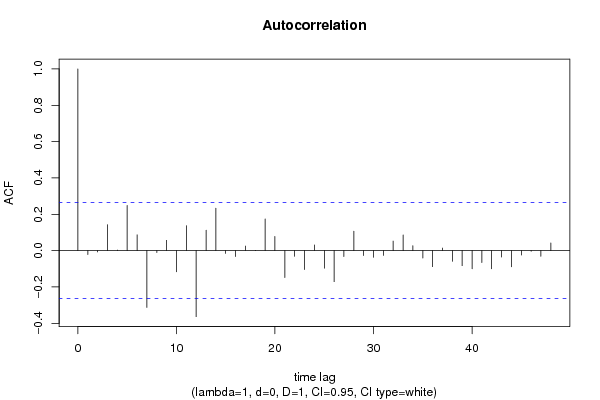
Title produced by software

(Partial) Autocorrelation Function

Date of computation

Tue, 07 Dec 2010 15:16:06 +0000

Cite this page as follows

Statistical Computations at FreeStatistics.org, Office for Research Development and Education, URL https://freestatistics.org/blog/index.php?v=date/2010/Dec/07/t1291734866oz7b7ediyiar2p9.htm/, Retrieved Sat, 04 May 2024 03:11:09 +0000

Statistical Computations at FreeStatistics.org, Office for Research Development and Education, URL https://freestatistics.org/blog/index.php?pk=106406, Retrieved Sat, 04 May 2024 03:11:09 +0000

QR Codes:

Paste this QR Code to cite your computation.

Original text written by user:

IsPrivate?

No (this computation is public)

User-defined keywords

Estimated Impact

146

Family? (F = Feedback message, R = changed R code, M = changed R Module, P = changed Parameters, D = changed Data)

-     [Univariate Data Series] [data set] [2008-12-01 19:54:57] [b98453cac15ba1066b407e146608df68]
- RMP   [(Partial) Autocorrelation Function] [Unemployment] [2010-11-29 09:05:21] [b98453cac15ba1066b407e146608df68]
-    D    [(Partial) Autocorrelation Function] [ACF 1] [2010-12-06 22:52:14] [b8e188bcc949964bed729335b3416734]
-    D      [(Partial) Autocorrelation Function] [ACF 2] [2010-12-06 23:38:48] [b8e188bcc949964bed729335b3416734]
-   P         [(Partial) Autocorrelation Function] [ACF 2.1] [2010-12-06 23:51:36] [b8e188bcc949964bed729335b3416734]
-   P             [(Partial) Autocorrelation Function] [ACF 2.2] [2010-12-07 15:16:06] [278a0539dc236556c5f30b5bc56ff9eb] [Current]

Feedback Forum

Post a new message

Dataseries X:

Download CSV

Histogram

Boxplots

Summary of computational transaction
Raw Input	view raw input (R code)
Raw Output	view raw output of R engine
Computing time	6 seconds
R Server	'Sir Ronald Aylmer Fisher' @ 193.190.124.24

\begin{tabular}{lllllllll}
\hline
Summary of computational transaction \tabularnewline
Raw Input & view raw input (R code)  \tabularnewline
Raw Output & view raw output of R engine  \tabularnewline
Computing time & 6 seconds \tabularnewline
R Server & 'Sir Ronald Aylmer Fisher' @ 193.190.124.24 \tabularnewline
\hline
\end{tabular}
%Source: https://freestatistics.org/blog/index.php?pk=106406&T=0

[TABLE]
[ROW][C]Summary of computational transaction[/C][/ROW]
[ROW][C]Raw Input[/C][C]view raw input (R code) [/C][/ROW]
[ROW][C]Raw Output[/C][C]view raw output of R engine [/C][/ROW]
[ROW][C]Computing time[/C][C]6 seconds[/C][/ROW]
[ROW][C]R Server[/C][C]'Sir Ronald Aylmer Fisher' @ 193.190.124.24[/C][/ROW]
[/TABLE]
Source: https://freestatistics.org/blog/index.php?pk=106406&T=0

Globally Unique Identifier (entire table): ba.freestatistics.org/blog/index.php?pk=106406&T=0

As an alternative you can also use a QR Code:

The GUIDs for individual cells are displayed in the table below:

Summary of computational transaction
Raw Input	view raw input (R code)
Raw Output	view raw output of R engine
Computing time	6 seconds
R Server	'Sir Ronald Aylmer Fisher' @ 193.190.124.24

Autocorrelation Function
Time lag k	ACF(k)	T-STAT	P-value
1	-0.021843	-0.162	0.435951
2	-0.007143	-0.053	0.478973
3	0.14231	1.0554	0.147929
4	0.002768	0.0205	0.491848
5	0.248116	1.8401	0.035578
6	0.08682	0.6439	0.261167
7	-0.31281	-2.3199	0.012043
8	-0.010889	-0.0808	0.467964
9	0.056537	0.4193	0.338319
10	-0.116859	-0.8667	0.194949
11	0.137169	1.0173	0.156739
12	-0.363628	-2.6967	0.004638
13	0.112018	0.8307	0.204854
14	0.232971	1.7278	0.044821
15	-0.015316	-0.1136	0.454989
16	-0.032765	-0.243	0.404459
17	0.024794	0.1839	0.427394
18	-0.000852	-0.0063	0.497491
19	0.17401	1.2905	0.101139
20	0.077849	0.5773	0.283032
21	-0.148771	-1.1033	0.137346
22	-0.030786	-0.2283	0.410125
23	-0.104207	-0.7728	0.22147
24	0.031057	0.2303	0.409346
25	-0.096493	-0.7156	0.238629
26	-0.170958	-1.2679	0.105095
27	-0.032423	-0.2405	0.405436
28	0.106606	0.7906	0.216284
29	-0.027259	-0.2022	0.420269
30	-0.03641	-0.27	0.394077
31	-0.026481	-0.1964	0.422516
32	0.052387	0.3885	0.349568
33	0.08559	0.6348	0.264111
34	0.026582	0.1971	0.422225
35	-0.040574	-0.3009	0.38231
36	-0.08848	-0.6562	0.257221
37	0.013815	0.1025	0.459385
38	-0.059281	-0.4396	0.330959
39	-0.082779	-0.6139	0.270904
40	-0.100521	-0.7455	0.229576
41	-0.065894	-0.4887	0.313506
42	-0.099751	-0.7398	0.231291
43	-0.035466	-0.263	0.396759
44	-0.089529	-0.664	0.254743
45	-0.024573	-0.1822	0.428033
46	-0.004237	-0.0314	0.487524
47	-0.03105	-0.2303	0.409368
48	0.042264	0.3134	0.377566

\begin{tabular}{lllllllll}
\hline
Autocorrelation Function \tabularnewline
Time lag k & ACF(k) & T-STAT & P-value \tabularnewline
1 & -0.021843 & -0.162 & 0.435951 \tabularnewline
2 & -0.007143 & -0.053 & 0.478973 \tabularnewline
3 & 0.14231 & 1.0554 & 0.147929 \tabularnewline
4 & 0.002768 & 0.0205 & 0.491848 \tabularnewline
5 & 0.248116 & 1.8401 & 0.035578 \tabularnewline
6 & 0.08682 & 0.6439 & 0.261167 \tabularnewline
7 & -0.31281 & -2.3199 & 0.012043 \tabularnewline
8 & -0.010889 & -0.0808 & 0.467964 \tabularnewline
9 & 0.056537 & 0.4193 & 0.338319 \tabularnewline
10 & -0.116859 & -0.8667 & 0.194949 \tabularnewline
11 & 0.137169 & 1.0173 & 0.156739 \tabularnewline
12 & -0.363628 & -2.6967 & 0.004638 \tabularnewline
13 & 0.112018 & 0.8307 & 0.204854 \tabularnewline
14 & 0.232971 & 1.7278 & 0.044821 \tabularnewline
15 & -0.015316 & -0.1136 & 0.454989 \tabularnewline
16 & -0.032765 & -0.243 & 0.404459 \tabularnewline
17 & 0.024794 & 0.1839 & 0.427394 \tabularnewline
18 & -0.000852 & -0.0063 & 0.497491 \tabularnewline
19 & 0.17401 & 1.2905 & 0.101139 \tabularnewline
20 & 0.077849 & 0.5773 & 0.283032 \tabularnewline
21 & -0.148771 & -1.1033 & 0.137346 \tabularnewline
22 & -0.030786 & -0.2283 & 0.410125 \tabularnewline
23 & -0.104207 & -0.7728 & 0.22147 \tabularnewline
24 & 0.031057 & 0.2303 & 0.409346 \tabularnewline
25 & -0.096493 & -0.7156 & 0.238629 \tabularnewline
26 & -0.170958 & -1.2679 & 0.105095 \tabularnewline
27 & -0.032423 & -0.2405 & 0.405436 \tabularnewline
28 & 0.106606 & 0.7906 & 0.216284 \tabularnewline
29 & -0.027259 & -0.2022 & 0.420269 \tabularnewline
30 & -0.03641 & -0.27 & 0.394077 \tabularnewline
31 & -0.026481 & -0.1964 & 0.422516 \tabularnewline
32 & 0.052387 & 0.3885 & 0.349568 \tabularnewline
33 & 0.08559 & 0.6348 & 0.264111 \tabularnewline
34 & 0.026582 & 0.1971 & 0.422225 \tabularnewline
35 & -0.040574 & -0.3009 & 0.38231 \tabularnewline
36 & -0.08848 & -0.6562 & 0.257221 \tabularnewline
37 & 0.013815 & 0.1025 & 0.459385 \tabularnewline
38 & -0.059281 & -0.4396 & 0.330959 \tabularnewline
39 & -0.082779 & -0.6139 & 0.270904 \tabularnewline
40 & -0.100521 & -0.7455 & 0.229576 \tabularnewline
41 & -0.065894 & -0.4887 & 0.313506 \tabularnewline
42 & -0.099751 & -0.7398 & 0.231291 \tabularnewline
43 & -0.035466 & -0.263 & 0.396759 \tabularnewline
44 & -0.089529 & -0.664 & 0.254743 \tabularnewline
45 & -0.024573 & -0.1822 & 0.428033 \tabularnewline
46 & -0.004237 & -0.0314 & 0.487524 \tabularnewline
47 & -0.03105 & -0.2303 & 0.409368 \tabularnewline
48 & 0.042264 & 0.3134 & 0.377566 \tabularnewline
\hline
\end{tabular}
%Source: https://freestatistics.org/blog/index.php?pk=106406&T=1

[TABLE]
[ROW][C]Autocorrelation Function[/C][/ROW]
[ROW][C]Time lag k[/C][C]ACF(k)[/C][C]T-STAT[/C][C]P-value[/C][/ROW]
[ROW][C]1[/C][C]-0.021843[/C][C]-0.162[/C][C]0.435951[/C][/ROW]
[ROW][C]2[/C][C]-0.007143[/C][C]-0.053[/C][C]0.478973[/C][/ROW]
[ROW][C]3[/C][C]0.14231[/C][C]1.0554[/C][C]0.147929[/C][/ROW]
[ROW][C]4[/C][C]0.002768[/C][C]0.0205[/C][C]0.491848[/C][/ROW]
[ROW][C]5[/C][C]0.248116[/C][C]1.8401[/C][C]0.035578[/C][/ROW]
[ROW][C]6[/C][C]0.08682[/C][C]0.6439[/C][C]0.261167[/C][/ROW]
[ROW][C]7[/C][C]-0.31281[/C][C]-2.3199[/C][C]0.012043[/C][/ROW]
[ROW][C]8[/C][C]-0.010889[/C][C]-0.0808[/C][C]0.467964[/C][/ROW]
[ROW][C]9[/C][C]0.056537[/C][C]0.4193[/C][C]0.338319[/C][/ROW]
[ROW][C]10[/C][C]-0.116859[/C][C]-0.8667[/C][C]0.194949[/C][/ROW]
[ROW][C]11[/C][C]0.137169[/C][C]1.0173[/C][C]0.156739[/C][/ROW]
[ROW][C]12[/C][C]-0.363628[/C][C]-2.6967[/C][C]0.004638[/C][/ROW]
[ROW][C]13[/C][C]0.112018[/C][C]0.8307[/C][C]0.204854[/C][/ROW]
[ROW][C]14[/C][C]0.232971[/C][C]1.7278[/C][C]0.044821[/C][/ROW]
[ROW][C]15[/C][C]-0.015316[/C][C]-0.1136[/C][C]0.454989[/C][/ROW]
[ROW][C]16[/C][C]-0.032765[/C][C]-0.243[/C][C]0.404459[/C][/ROW]
[ROW][C]17[/C][C]0.024794[/C][C]0.1839[/C][C]0.427394[/C][/ROW]
[ROW][C]18[/C][C]-0.000852[/C][C]-0.0063[/C][C]0.497491[/C][/ROW]
[ROW][C]19[/C][C]0.17401[/C][C]1.2905[/C][C]0.101139[/C][/ROW]
[ROW][C]20[/C][C]0.077849[/C][C]0.5773[/C][C]0.283032[/C][/ROW]
[ROW][C]21[/C][C]-0.148771[/C][C]-1.1033[/C][C]0.137346[/C][/ROW]
[ROW][C]22[/C][C]-0.030786[/C][C]-0.2283[/C][C]0.410125[/C][/ROW]
[ROW][C]23[/C][C]-0.104207[/C][C]-0.7728[/C][C]0.22147[/C][/ROW]
[ROW][C]24[/C][C]0.031057[/C][C]0.2303[/C][C]0.409346[/C][/ROW]
[ROW][C]25[/C][C]-0.096493[/C][C]-0.7156[/C][C]0.238629[/C][/ROW]
[ROW][C]26[/C][C]-0.170958[/C][C]-1.2679[/C][C]0.105095[/C][/ROW]
[ROW][C]27[/C][C]-0.032423[/C][C]-0.2405[/C][C]0.405436[/C][/ROW]
[ROW][C]28[/C][C]0.106606[/C][C]0.7906[/C][C]0.216284[/C][/ROW]
[ROW][C]29[/C][C]-0.027259[/C][C]-0.2022[/C][C]0.420269[/C][/ROW]
[ROW][C]30[/C][C]-0.03641[/C][C]-0.27[/C][C]0.394077[/C][/ROW]
[ROW][C]31[/C][C]-0.026481[/C][C]-0.1964[/C][C]0.422516[/C][/ROW]
[ROW][C]32[/C][C]0.052387[/C][C]0.3885[/C][C]0.349568[/C][/ROW]
[ROW][C]33[/C][C]0.08559[/C][C]0.6348[/C][C]0.264111[/C][/ROW]
[ROW][C]34[/C][C]0.026582[/C][C]0.1971[/C][C]0.422225[/C][/ROW]
[ROW][C]35[/C][C]-0.040574[/C][C]-0.3009[/C][C]0.38231[/C][/ROW]
[ROW][C]36[/C][C]-0.08848[/C][C]-0.6562[/C][C]0.257221[/C][/ROW]
[ROW][C]37[/C][C]0.013815[/C][C]0.1025[/C][C]0.459385[/C][/ROW]
[ROW][C]38[/C][C]-0.059281[/C][C]-0.4396[/C][C]0.330959[/C][/ROW]
[ROW][C]39[/C][C]-0.082779[/C][C]-0.6139[/C][C]0.270904[/C][/ROW]
[ROW][C]40[/C][C]-0.100521[/C][C]-0.7455[/C][C]0.229576[/C][/ROW]
[ROW][C]41[/C][C]-0.065894[/C][C]-0.4887[/C][C]0.313506[/C][/ROW]
[ROW][C]42[/C][C]-0.099751[/C][C]-0.7398[/C][C]0.231291[/C][/ROW]
[ROW][C]43[/C][C]-0.035466[/C][C]-0.263[/C][C]0.396759[/C][/ROW]
[ROW][C]44[/C][C]-0.089529[/C][C]-0.664[/C][C]0.254743[/C][/ROW]
[ROW][C]45[/C][C]-0.024573[/C][C]-0.1822[/C][C]0.428033[/C][/ROW]
[ROW][C]46[/C][C]-0.004237[/C][C]-0.0314[/C][C]0.487524[/C][/ROW]
[ROW][C]47[/C][C]-0.03105[/C][C]-0.2303[/C][C]0.409368[/C][/ROW]
[ROW][C]48[/C][C]0.042264[/C][C]0.3134[/C][C]0.377566[/C][/ROW]
[/TABLE]
Source: https://freestatistics.org/blog/index.php?pk=106406&T=1

Globally Unique Identifier (entire table): ba.freestatistics.org/blog/index.php?pk=106406&T=1

As an alternative you can also use a QR Code:

The GUIDs for individual cells are displayed in the table below:

Autocorrelation Function
Time lag k	ACF(k)	T-STAT	P-value
1	-0.021843	-0.162	0.435951
2	-0.007143	-0.053	0.478973
3	0.14231	1.0554	0.147929
4	0.002768	0.0205	0.491848
5	0.248116	1.8401	0.035578
6	0.08682	0.6439	0.261167
7	-0.31281	-2.3199	0.012043
8	-0.010889	-0.0808	0.467964
9	0.056537	0.4193	0.338319
10	-0.116859	-0.8667	0.194949
11	0.137169	1.0173	0.156739
12	-0.363628	-2.6967	0.004638
13	0.112018	0.8307	0.204854
14	0.232971	1.7278	0.044821
15	-0.015316	-0.1136	0.454989
16	-0.032765	-0.243	0.404459
17	0.024794	0.1839	0.427394
18	-0.000852	-0.0063	0.497491
19	0.17401	1.2905	0.101139
20	0.077849	0.5773	0.283032
21	-0.148771	-1.1033	0.137346
22	-0.030786	-0.2283	0.410125
23	-0.104207	-0.7728	0.22147
24	0.031057	0.2303	0.409346
25	-0.096493	-0.7156	0.238629
26	-0.170958	-1.2679	0.105095
27	-0.032423	-0.2405	0.405436
28	0.106606	0.7906	0.216284
29	-0.027259	-0.2022	0.420269
30	-0.03641	-0.27	0.394077
31	-0.026481	-0.1964	0.422516
32	0.052387	0.3885	0.349568
33	0.08559	0.6348	0.264111
34	0.026582	0.1971	0.422225
35	-0.040574	-0.3009	0.38231
36	-0.08848	-0.6562	0.257221
37	0.013815	0.1025	0.459385
38	-0.059281	-0.4396	0.330959
39	-0.082779	-0.6139	0.270904
40	-0.100521	-0.7455	0.229576
41	-0.065894	-0.4887	0.313506
42	-0.099751	-0.7398	0.231291
43	-0.035466	-0.263	0.396759
44	-0.089529	-0.664	0.254743
45	-0.024573	-0.1822	0.428033
46	-0.004237	-0.0314	0.487524
47	-0.03105	-0.2303	0.409368
48	0.042264	0.3134	0.377566

Partial Autocorrelation Function
Time lag k	PACF(k)	T-STAT	P-value
1	-0.021843	-0.162	0.435951
2	-0.007624	-0.0565	0.477559
3	0.142062	1.0536	0.148345
4	0.009004	0.0668	0.473503
5	0.255332	1.8936	0.031772
6	0.085527	0.6343	0.264262
7	-0.327506	-2.4289	0.009221
8	-0.118095	-0.8758	0.19247
9	0.03002	0.2226	0.412321
10	-0.105688	-0.7838	0.218259
11	0.154153	1.1432	0.128947
12	-0.255383	-1.894	0.031746
13	0.26853	1.9915	0.025702
14	0.145401	1.0783	0.142798
15	0.084853	0.6293	0.265882
16	-0.118991	-0.8825	0.190684
17	0.021307	0.158	0.437511
18	-0.00324	-0.024	0.490459
19	-0.09385	-0.696	0.244677
20	0.063683	0.4723	0.319296
21	0.043593	0.3233	0.373849
22	-0.150038	-1.1127	0.135337
23	-0.068413	-0.5074	0.306964
24	-0.110343	-0.8183	0.208351
25	-0.01188	-0.0881	0.465058
26	-0.067458	-0.5003	0.309438
27	0.097119	0.7203	0.23721
28	0.153249	1.1365	0.130333
29	0.043834	0.3251	0.373176
30	-0.034145	-0.2532	0.400519
31	-0.069074	-0.5123	0.305259
32	0.046252	0.343	0.366447
33	-0.144523	-1.0718	0.144243
34	-0.083076	-0.6161	0.270183
35	0.003843	0.0285	0.488683
36	-0.009719	-0.0721	0.4714
37	-0.011272	-0.0836	0.466842
38	-0.130606	-0.9686	0.168492
39	0.006135	0.0455	0.481938
40	0.024366	0.1807	0.428632
41	-0.061781	-0.4582	0.324315
42	-0.121062	-0.8978	0.186597
43	0.015445	0.1145	0.454612
44	0.078803	0.5844	0.280665
45	-0.069272	-0.5137	0.304749
46	-0.061054	-0.4528	0.326242
47	-0.029381	-0.2179	0.414158
48	-0.059395	-0.4405	0.330657

\begin{tabular}{lllllllll}
\hline
Partial Autocorrelation Function \tabularnewline
Time lag k & PACF(k) & T-STAT & P-value \tabularnewline
1 & -0.021843 & -0.162 & 0.435951 \tabularnewline
2 & -0.007624 & -0.0565 & 0.477559 \tabularnewline
3 & 0.142062 & 1.0536 & 0.148345 \tabularnewline
4 & 0.009004 & 0.0668 & 0.473503 \tabularnewline
5 & 0.255332 & 1.8936 & 0.031772 \tabularnewline
6 & 0.085527 & 0.6343 & 0.264262 \tabularnewline
7 & -0.327506 & -2.4289 & 0.009221 \tabularnewline
8 & -0.118095 & -0.8758 & 0.19247 \tabularnewline
9 & 0.03002 & 0.2226 & 0.412321 \tabularnewline
10 & -0.105688 & -0.7838 & 0.218259 \tabularnewline
11 & 0.154153 & 1.1432 & 0.128947 \tabularnewline
12 & -0.255383 & -1.894 & 0.031746 \tabularnewline
13 & 0.26853 & 1.9915 & 0.025702 \tabularnewline
14 & 0.145401 & 1.0783 & 0.142798 \tabularnewline
15 & 0.084853 & 0.6293 & 0.265882 \tabularnewline
16 & -0.118991 & -0.8825 & 0.190684 \tabularnewline
17 & 0.021307 & 0.158 & 0.437511 \tabularnewline
18 & -0.00324 & -0.024 & 0.490459 \tabularnewline
19 & -0.09385 & -0.696 & 0.244677 \tabularnewline
20 & 0.063683 & 0.4723 & 0.319296 \tabularnewline
21 & 0.043593 & 0.3233 & 0.373849 \tabularnewline
22 & -0.150038 & -1.1127 & 0.135337 \tabularnewline
23 & -0.068413 & -0.5074 & 0.306964 \tabularnewline
24 & -0.110343 & -0.8183 & 0.208351 \tabularnewline
25 & -0.01188 & -0.0881 & 0.465058 \tabularnewline
26 & -0.067458 & -0.5003 & 0.309438 \tabularnewline
27 & 0.097119 & 0.7203 & 0.23721 \tabularnewline
28 & 0.153249 & 1.1365 & 0.130333 \tabularnewline
29 & 0.043834 & 0.3251 & 0.373176 \tabularnewline
30 & -0.034145 & -0.2532 & 0.400519 \tabularnewline
31 & -0.069074 & -0.5123 & 0.305259 \tabularnewline
32 & 0.046252 & 0.343 & 0.366447 \tabularnewline
33 & -0.144523 & -1.0718 & 0.144243 \tabularnewline
34 & -0.083076 & -0.6161 & 0.270183 \tabularnewline
35 & 0.003843 & 0.0285 & 0.488683 \tabularnewline
36 & -0.009719 & -0.0721 & 0.4714 \tabularnewline
37 & -0.011272 & -0.0836 & 0.466842 \tabularnewline
38 & -0.130606 & -0.9686 & 0.168492 \tabularnewline
39 & 0.006135 & 0.0455 & 0.481938 \tabularnewline
40 & 0.024366 & 0.1807 & 0.428632 \tabularnewline
41 & -0.061781 & -0.4582 & 0.324315 \tabularnewline
42 & -0.121062 & -0.8978 & 0.186597 \tabularnewline
43 & 0.015445 & 0.1145 & 0.454612 \tabularnewline
44 & 0.078803 & 0.5844 & 0.280665 \tabularnewline
45 & -0.069272 & -0.5137 & 0.304749 \tabularnewline
46 & -0.061054 & -0.4528 & 0.326242 \tabularnewline
47 & -0.029381 & -0.2179 & 0.414158 \tabularnewline
48 & -0.059395 & -0.4405 & 0.330657 \tabularnewline
\hline
\end{tabular}
%Source: https://freestatistics.org/blog/index.php?pk=106406&T=2

[TABLE]
[ROW][C]Partial Autocorrelation Function[/C][/ROW]
[ROW][C]Time lag k[/C][C]PACF(k)[/C][C]T-STAT[/C][C]P-value[/C][/ROW]
[ROW][C]1[/C][C]-0.021843[/C][C]-0.162[/C][C]0.435951[/C][/ROW]
[ROW][C]2[/C][C]-0.007624[/C][C]-0.0565[/C][C]0.477559[/C][/ROW]
[ROW][C]3[/C][C]0.142062[/C][C]1.0536[/C][C]0.148345[/C][/ROW]
[ROW][C]4[/C][C]0.009004[/C][C]0.0668[/C][C]0.473503[/C][/ROW]
[ROW][C]5[/C][C]0.255332[/C][C]1.8936[/C][C]0.031772[/C][/ROW]
[ROW][C]6[/C][C]0.085527[/C][C]0.6343[/C][C]0.264262[/C][/ROW]
[ROW][C]7[/C][C]-0.327506[/C][C]-2.4289[/C][C]0.009221[/C][/ROW]
[ROW][C]8[/C][C]-0.118095[/C][C]-0.8758[/C][C]0.19247[/C][/ROW]
[ROW][C]9[/C][C]0.03002[/C][C]0.2226[/C][C]0.412321[/C][/ROW]
[ROW][C]10[/C][C]-0.105688[/C][C]-0.7838[/C][C]0.218259[/C][/ROW]
[ROW][C]11[/C][C]0.154153[/C][C]1.1432[/C][C]0.128947[/C][/ROW]
[ROW][C]12[/C][C]-0.255383[/C][C]-1.894[/C][C]0.031746[/C][/ROW]
[ROW][C]13[/C][C]0.26853[/C][C]1.9915[/C][C]0.025702[/C][/ROW]
[ROW][C]14[/C][C]0.145401[/C][C]1.0783[/C][C]0.142798[/C][/ROW]
[ROW][C]15[/C][C]0.084853[/C][C]0.6293[/C][C]0.265882[/C][/ROW]
[ROW][C]16[/C][C]-0.118991[/C][C]-0.8825[/C][C]0.190684[/C][/ROW]
[ROW][C]17[/C][C]0.021307[/C][C]0.158[/C][C]0.437511[/C][/ROW]
[ROW][C]18[/C][C]-0.00324[/C][C]-0.024[/C][C]0.490459[/C][/ROW]
[ROW][C]19[/C][C]-0.09385[/C][C]-0.696[/C][C]0.244677[/C][/ROW]
[ROW][C]20[/C][C]0.063683[/C][C]0.4723[/C][C]0.319296[/C][/ROW]
[ROW][C]21[/C][C]0.043593[/C][C]0.3233[/C][C]0.373849[/C][/ROW]
[ROW][C]22[/C][C]-0.150038[/C][C]-1.1127[/C][C]0.135337[/C][/ROW]
[ROW][C]23[/C][C]-0.068413[/C][C]-0.5074[/C][C]0.306964[/C][/ROW]
[ROW][C]24[/C][C]-0.110343[/C][C]-0.8183[/C][C]0.208351[/C][/ROW]
[ROW][C]25[/C][C]-0.01188[/C][C]-0.0881[/C][C]0.465058[/C][/ROW]
[ROW][C]26[/C][C]-0.067458[/C][C]-0.5003[/C][C]0.309438[/C][/ROW]
[ROW][C]27[/C][C]0.097119[/C][C]0.7203[/C][C]0.23721[/C][/ROW]
[ROW][C]28[/C][C]0.153249[/C][C]1.1365[/C][C]0.130333[/C][/ROW]
[ROW][C]29[/C][C]0.043834[/C][C]0.3251[/C][C]0.373176[/C][/ROW]
[ROW][C]30[/C][C]-0.034145[/C][C]-0.2532[/C][C]0.400519[/C][/ROW]
[ROW][C]31[/C][C]-0.069074[/C][C]-0.5123[/C][C]0.305259[/C][/ROW]
[ROW][C]32[/C][C]0.046252[/C][C]0.343[/C][C]0.366447[/C][/ROW]
[ROW][C]33[/C][C]-0.144523[/C][C]-1.0718[/C][C]0.144243[/C][/ROW]
[ROW][C]34[/C][C]-0.083076[/C][C]-0.6161[/C][C]0.270183[/C][/ROW]
[ROW][C]35[/C][C]0.003843[/C][C]0.0285[/C][C]0.488683[/C][/ROW]
[ROW][C]36[/C][C]-0.009719[/C][C]-0.0721[/C][C]0.4714[/C][/ROW]
[ROW][C]37[/C][C]-0.011272[/C][C]-0.0836[/C][C]0.466842[/C][/ROW]
[ROW][C]38[/C][C]-0.130606[/C][C]-0.9686[/C][C]0.168492[/C][/ROW]
[ROW][C]39[/C][C]0.006135[/C][C]0.0455[/C][C]0.481938[/C][/ROW]
[ROW][C]40[/C][C]0.024366[/C][C]0.1807[/C][C]0.428632[/C][/ROW]
[ROW][C]41[/C][C]-0.061781[/C][C]-0.4582[/C][C]0.324315[/C][/ROW]
[ROW][C]42[/C][C]-0.121062[/C][C]-0.8978[/C][C]0.186597[/C][/ROW]
[ROW][C]43[/C][C]0.015445[/C][C]0.1145[/C][C]0.454612[/C][/ROW]
[ROW][C]44[/C][C]0.078803[/C][C]0.5844[/C][C]0.280665[/C][/ROW]
[ROW][C]45[/C][C]-0.069272[/C][C]-0.5137[/C][C]0.304749[/C][/ROW]
[ROW][C]46[/C][C]-0.061054[/C][C]-0.4528[/C][C]0.326242[/C][/ROW]
[ROW][C]47[/C][C]-0.029381[/C][C]-0.2179[/C][C]0.414158[/C][/ROW]
[ROW][C]48[/C][C]-0.059395[/C][C]-0.4405[/C][C]0.330657[/C][/ROW]
[/TABLE]
Source: https://freestatistics.org/blog/index.php?pk=106406&T=2

Globally Unique Identifier (entire table): ba.freestatistics.org/blog/index.php?pk=106406&T=2

As an alternative you can also use a QR Code:

The GUIDs for individual cells are displayed in the table below:

Partial Autocorrelation Function
Time lag k	PACF(k)	T-STAT	P-value
1	-0.021843	-0.162	0.435951
2	-0.007624	-0.0565	0.477559
3	0.142062	1.0536	0.148345
4	0.009004	0.0668	0.473503
5	0.255332	1.8936	0.031772
6	0.085527	0.6343	0.264262
7	-0.327506	-2.4289	0.009221
8	-0.118095	-0.8758	0.19247
9	0.03002	0.2226	0.412321
10	-0.105688	-0.7838	0.218259
11	0.154153	1.1432	0.128947
12	-0.255383	-1.894	0.031746
13	0.26853	1.9915	0.025702
14	0.145401	1.0783	0.142798
15	0.084853	0.6293	0.265882
16	-0.118991	-0.8825	0.190684
17	0.021307	0.158	0.437511
18	-0.00324	-0.024	0.490459
19	-0.09385	-0.696	0.244677
20	0.063683	0.4723	0.319296
21	0.043593	0.3233	0.373849
22	-0.150038	-1.1127	0.135337
23	-0.068413	-0.5074	0.306964
24	-0.110343	-0.8183	0.208351
25	-0.01188	-0.0881	0.465058
26	-0.067458	-0.5003	0.309438
27	0.097119	0.7203	0.23721
28	0.153249	1.1365	0.130333
29	0.043834	0.3251	0.373176
30	-0.034145	-0.2532	0.400519
31	-0.069074	-0.5123	0.305259
32	0.046252	0.343	0.366447
33	-0.144523	-1.0718	0.144243
34	-0.083076	-0.6161	0.270183
35	0.003843	0.0285	0.488683
36	-0.009719	-0.0721	0.4714
37	-0.011272	-0.0836	0.466842
38	-0.130606	-0.9686	0.168492
39	0.006135	0.0455	0.481938
40	0.024366	0.1807	0.428632
41	-0.061781	-0.4582	0.324315
42	-0.121062	-0.8978	0.186597
43	0.015445	0.1145	0.454612
44	0.078803	0.5844	0.280665
45	-0.069272	-0.5137	0.304749
46	-0.061054	-0.4528	0.326242
47	-0.029381	-0.2179	0.414158
48	-0.059395	-0.4405	0.330657

Figure 1

PNG link

Postscript link

PDF link

Figure 2

PNG link

Postscript link

PDF link

Parameters (Session):

par1 = 48 ; par2 = 1 ; par3 = 0 ; par4 = 1 ; par5 = 12 ; par6 = White Noise ; par7 = 0.95 ;

Parameters (R input):

par1 = 48 ; par2 = 1 ; par3 = 0 ; par4 = 1 ; par5 = 12 ; par6 = White Noise ; par7 = 0.95 ;

R code (references can be found in the software module):

if (par1 == 'Default') {
par1 = 10*log10(length(x))
} else {
par1 <- as.numeric(par1)
}
par2 <- as.numeric(par2)
par3 <- as.numeric(par3)
par4 <- as.numeric(par4)
par5 <- as.numeric(par5)
if (par6 == 'White Noise') par6 <- 'white' else par6 <- 'ma'
par7 <- as.numeric(par7)
if (par2 == 0) {
x <- log(x)
} else {
x <- (x ^ par2 - 1) / par2
}
if (par3 > 0) x <- diff(x,lag=1,difference=par3)
if (par4 > 0) x <- diff(x,lag=par5,difference=par4)
bitmap(file='pic1.png')
racf <- acf(x, par1, main='Autocorrelation', xlab='time lag', ylab='ACF', ci.type=par6, ci=par7, sub=paste('(lambda=',par2,', d=',par3,', D=',par4,', CI=', par7, ', CI type=',par6,')',sep=''))
dev.off()
bitmap(file='pic2.png')
rpacf <- pacf(x,par1,main='Partial Autocorrelation',xlab='lags',ylab='PACF')
dev.off()
(myacf <- c(racf$acf))
(mypacf <- c(rpacf$acf))
lengthx <- length(x)
sqrtn <- sqrt(lengthx)
load(file='createtable')
a<-table.start()
a<-table.row.start(a)
a<-table.element(a,'Autocorrelation Function',4,TRUE)
a<-table.row.end(a)
a<-table.row.start(a)
a<-table.element(a,'Time lag k',header=TRUE)
a<-table.element(a,hyperlink('basics.htm','ACF(k)','click here for more information about the Autocorrelation Function'),header=TRUE)
a<-table.element(a,'T-STAT',header=TRUE)
a<-table.element(a,'P-value',header=TRUE)
a<-table.row.end(a)
for (i in 2:(par1+1)) {
a<-table.row.start(a)
a<-table.element(a,i-1,header=TRUE)
a<-table.element(a,round(myacf[i],6))
mytstat <- myacf[i]*sqrtn
a<-table.element(a,round(mytstat,4))
a<-table.element(a,round(1-pt(abs(mytstat),lengthx),6))
a<-table.row.end(a)
}
a<-table.end(a)
table.save(a,file='mytable.tab')
a<-table.start()
a<-table.row.start(a)
a<-table.element(a,'Partial Autocorrelation Function',4,TRUE)
a<-table.row.end(a)
a<-table.row.start(a)
a<-table.element(a,'Time lag k',header=TRUE)
a<-table.element(a,hyperlink('basics.htm','PACF(k)','click here for more information about the Partial Autocorrelation Function'),header=TRUE)
a<-table.element(a,'T-STAT',header=TRUE)
a<-table.element(a,'P-value',header=TRUE)
a<-table.row.end(a)
for (i in 1:par1) {
a<-table.row.start(a)
a<-table.element(a,i,header=TRUE)
a<-table.element(a,round(mypacf[i],6))
mytstat <- mypacf[i]*sqrtn
a<-table.element(a,round(mytstat,4))
a<-table.element(a,round(1-pt(abs(mytstat),lengthx),6))
a<-table.row.end(a)
}
a<-table.end(a)
table.save(a,file='mytable1.tab')

Free Statistics

Description of Statistical Computation

Tree of Dependent Computations

Dataset

Tables (Output of Computation)

Figures (Output of Computation)

Input Parameters & R Code