Repository of Reproducible Computations

Free Statistics

of Irreproducible Research!

Author's title

Author

*The author of this computation has been verified*

R Software Module

rwasp_autocorrelation.wasp

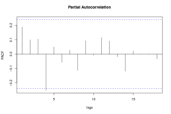
Title produced by software

(Partial) Autocorrelation Function

Date of computation

Mon, 06 Dec 2010 22:52:14 +0000

Cite this page as follows

Statistical Computations at FreeStatistics.org, Office for Research Development and Education, URL https://freestatistics.org/blog/index.php?v=date/2010/Dec/06/t12916758559ynqjjjk3j4oa57.htm/, Retrieved Sun, 28 Apr 2024 22:30:14 +0000

Statistical Computations at FreeStatistics.org, Office for Research Development and Education, URL https://freestatistics.org/blog/index.php?pk=105962, Retrieved Sun, 28 Apr 2024 22:30:14 +0000

QR Codes:

Paste this QR Code to cite your computation.

Original text written by user:

IsPrivate?

No (this computation is public)

User-defined keywords

Estimated Impact

157

Family? (F = Feedback message, R = changed R code, M = changed R Module, P = changed Parameters, D = changed Data)

-     [Univariate Data Series] [data set] [2008-12-01 19:54:57] [b98453cac15ba1066b407e146608df68]
- RMP   [(Partial) Autocorrelation Function] [Unemployment] [2010-11-29 09:05:21] [b98453cac15ba1066b407e146608df68]
-    D      [(Partial) Autocorrelation Function] [ACF 1] [2010-12-06 22:52:14] [278a0539dc236556c5f30b5bc56ff9eb] [Current]
-    D        [(Partial) Autocorrelation Function] [ACF 2] [2010-12-06 23:38:48] [b8e188bcc949964bed729335b3416734] 
-   P           [(Partial) Autocorrelation Function] [ACF 2.1] [2010-12-06 23:51:36] [b8e188bcc949964bed729335b3416734] 
-   P             [(Partial) Autocorrelation Function] [ACF 2.2] [2010-12-07 15:16:06] [b8e188bcc949964bed729335b3416734] 
-   P         [(Partial) Autocorrelation Function] [ACF 1.1] [2010-12-07 15:23:27] [b8e188bcc949964bed729335b3416734] 
-    D        [(Partial) Autocorrelation Function] [ACF Nieuwbouw] [2010-12-19 14:56:25] [b8e188bcc949964bed729335b3416734] 
-   P           [(Partial) Autocorrelation Function] [ACF Nieuwbouw] [2010-12-19 15:50:37] [b8e188bcc949964bed729335b3416734] 
-   P             [(Partial) Autocorrelation Function] [ACF Nieuwbouw 1] [2010-12-19 15:57:46] [b8e188bcc949964bed729335b3416734] 

Feedback Forum

Post a new message

Dataseries X:

Download CSV

Histogram

Boxplots

Summary of computational transaction
Raw Input	view raw input (R code)
Raw Output	view raw output of R engine
Computing time	1 seconds
R Server	'Gwilym Jenkins' @ 72.249.127.135

\begin{tabular}{lllllllll}
\hline
Summary of computational transaction \tabularnewline
Raw Input & view raw input (R code)  \tabularnewline
Raw Output & view raw output of R engine  \tabularnewline
Computing time & 1 seconds \tabularnewline
R Server & 'Gwilym Jenkins' @ 72.249.127.135 \tabularnewline
\hline
\end{tabular}
%Source: https://freestatistics.org/blog/index.php?pk=105962&T=0

[TABLE]
[ROW][C]Summary of computational transaction[/C][/ROW]
[ROW][C]Raw Input[/C][C]view raw input (R code) [/C][/ROW]
[ROW][C]Raw Output[/C][C]view raw output of R engine [/C][/ROW]
[ROW][C]Computing time[/C][C]1 seconds[/C][/ROW]
[ROW][C]R Server[/C][C]'Gwilym Jenkins' @ 72.249.127.135[/C][/ROW]
[/TABLE]
Source: https://freestatistics.org/blog/index.php?pk=105962&T=0

Globally Unique Identifier (entire table): ba.freestatistics.org/blog/index.php?pk=105962&T=0

As an alternative you can also use a QR Code:

The GUIDs for individual cells are displayed in the table below:

Summary of computational transaction
Raw Input	view raw input (R code)
Raw Output	view raw output of R engine
Computing time	1 seconds
R Server	'Gwilym Jenkins' @ 72.249.127.135

Autocorrelation Function
Time lag k	ACF(k)	T-STAT	P-value
1	0.189781	1.5534	0.062517
2	0.132304	1.083	0.141356
3	0.141837	1.161	0.124884
4	-0.183817	-1.5046	0.068563
5	-0.003948	-0.0323	0.487158
6	-0.073902	-0.6049	0.273639
7	-0.057234	-0.4685	0.320481
8	-0.065338	-0.5348	0.297273
9	0.015507	0.1269	0.449688
10	0.022253	0.1821	0.428008
11	0.086568	0.7086	0.240518
12	0.177692	1.4545	0.075243
13	0.029909	0.2448	0.403674
14	-0.034214	-0.2801	0.390149
15	-0.009241	-0.0756	0.469965
16	-0.064106	-0.5247	0.300751
17	-0.04218	-0.3453	0.36549
18	-0.023966	-0.1962	0.422537

\begin{tabular}{lllllllll}
\hline
Autocorrelation Function \tabularnewline
Time lag k & ACF(k) & T-STAT & P-value \tabularnewline
1 & 0.189781 & 1.5534 & 0.062517 \tabularnewline
2 & 0.132304 & 1.083 & 0.141356 \tabularnewline
3 & 0.141837 & 1.161 & 0.124884 \tabularnewline
4 & -0.183817 & -1.5046 & 0.068563 \tabularnewline
5 & -0.003948 & -0.0323 & 0.487158 \tabularnewline
6 & -0.073902 & -0.6049 & 0.273639 \tabularnewline
7 & -0.057234 & -0.4685 & 0.320481 \tabularnewline
8 & -0.065338 & -0.5348 & 0.297273 \tabularnewline
9 & 0.015507 & 0.1269 & 0.449688 \tabularnewline
10 & 0.022253 & 0.1821 & 0.428008 \tabularnewline
11 & 0.086568 & 0.7086 & 0.240518 \tabularnewline
12 & 0.177692 & 1.4545 & 0.075243 \tabularnewline
13 & 0.029909 & 0.2448 & 0.403674 \tabularnewline
14 & -0.034214 & -0.2801 & 0.390149 \tabularnewline
15 & -0.009241 & -0.0756 & 0.469965 \tabularnewline
16 & -0.064106 & -0.5247 & 0.300751 \tabularnewline
17 & -0.04218 & -0.3453 & 0.36549 \tabularnewline
18 & -0.023966 & -0.1962 & 0.422537 \tabularnewline
\hline
\end{tabular}
%Source: https://freestatistics.org/blog/index.php?pk=105962&T=1

[TABLE]
[ROW][C]Autocorrelation Function[/C][/ROW]
[ROW][C]Time lag k[/C][C]ACF(k)[/C][C]T-STAT[/C][C]P-value[/C][/ROW]
[ROW][C]1[/C][C]0.189781[/C][C]1.5534[/C][C]0.062517[/C][/ROW]
[ROW][C]2[/C][C]0.132304[/C][C]1.083[/C][C]0.141356[/C][/ROW]
[ROW][C]3[/C][C]0.141837[/C][C]1.161[/C][C]0.124884[/C][/ROW]
[ROW][C]4[/C][C]-0.183817[/C][C]-1.5046[/C][C]0.068563[/C][/ROW]
[ROW][C]5[/C][C]-0.003948[/C][C]-0.0323[/C][C]0.487158[/C][/ROW]
[ROW][C]6[/C][C]-0.073902[/C][C]-0.6049[/C][C]0.273639[/C][/ROW]
[ROW][C]7[/C][C]-0.057234[/C][C]-0.4685[/C][C]0.320481[/C][/ROW]
[ROW][C]8[/C][C]-0.065338[/C][C]-0.5348[/C][C]0.297273[/C][/ROW]
[ROW][C]9[/C][C]0.015507[/C][C]0.1269[/C][C]0.449688[/C][/ROW]
[ROW][C]10[/C][C]0.022253[/C][C]0.1821[/C][C]0.428008[/C][/ROW]
[ROW][C]11[/C][C]0.086568[/C][C]0.7086[/C][C]0.240518[/C][/ROW]
[ROW][C]12[/C][C]0.177692[/C][C]1.4545[/C][C]0.075243[/C][/ROW]
[ROW][C]13[/C][C]0.029909[/C][C]0.2448[/C][C]0.403674[/C][/ROW]
[ROW][C]14[/C][C]-0.034214[/C][C]-0.2801[/C][C]0.390149[/C][/ROW]
[ROW][C]15[/C][C]-0.009241[/C][C]-0.0756[/C][C]0.469965[/C][/ROW]
[ROW][C]16[/C][C]-0.064106[/C][C]-0.5247[/C][C]0.300751[/C][/ROW]
[ROW][C]17[/C][C]-0.04218[/C][C]-0.3453[/C][C]0.36549[/C][/ROW]
[ROW][C]18[/C][C]-0.023966[/C][C]-0.1962[/C][C]0.422537[/C][/ROW]
[/TABLE]
Source: https://freestatistics.org/blog/index.php?pk=105962&T=1

Globally Unique Identifier (entire table): ba.freestatistics.org/blog/index.php?pk=105962&T=1

As an alternative you can also use a QR Code:

The GUIDs for individual cells are displayed in the table below:

Autocorrelation Function
Time lag k	ACF(k)	T-STAT	P-value
1	0.189781	1.5534	0.062517
2	0.132304	1.083	0.141356
3	0.141837	1.161	0.124884
4	-0.183817	-1.5046	0.068563
5	-0.003948	-0.0323	0.487158
6	-0.073902	-0.6049	0.273639
7	-0.057234	-0.4685	0.320481
8	-0.065338	-0.5348	0.297273
9	0.015507	0.1269	0.449688
10	0.022253	0.1821	0.428008
11	0.086568	0.7086	0.240518
12	0.177692	1.4545	0.075243
13	0.029909	0.2448	0.403674
14	-0.034214	-0.2801	0.390149
15	-0.009241	-0.0756	0.469965
16	-0.064106	-0.5247	0.300751
17	-0.04218	-0.3453	0.36549
18	-0.023966	-0.1962	0.422537

Partial Autocorrelation Function
Time lag k	PACF(k)	T-STAT	P-value
1	0.189781	1.5534	0.062517
2	0.099884	0.8176	0.208245
3	0.105075	0.8601	0.196407
4	-0.251464	-2.0583	0.021726
5	0.050131	0.4103	0.341432
6	-0.057267	-0.4687	0.320385
7	0.027566	0.2256	0.411085
8	-0.114163	-0.9345	0.176711
9	0.093092	0.762	0.224371
10	-0.008887	-0.0727	0.471115
11	0.114583	0.9379	0.175833
12	0.091857	0.7519	0.227377
13	-0.018832	-0.1541	0.438979
14	-0.11937	-0.9771	0.166022
15	0.022267	0.1823	0.427963
16	-0.001587	-0.013	0.494836
17	0.001811	0.0148	0.494109
18	-0.033446	-0.2738	0.392553

\begin{tabular}{lllllllll}
\hline
Partial Autocorrelation Function \tabularnewline
Time lag k & PACF(k) & T-STAT & P-value \tabularnewline
1 & 0.189781 & 1.5534 & 0.062517 \tabularnewline
2 & 0.099884 & 0.8176 & 0.208245 \tabularnewline
3 & 0.105075 & 0.8601 & 0.196407 \tabularnewline
4 & -0.251464 & -2.0583 & 0.021726 \tabularnewline
5 & 0.050131 & 0.4103 & 0.341432 \tabularnewline
6 & -0.057267 & -0.4687 & 0.320385 \tabularnewline
7 & 0.027566 & 0.2256 & 0.411085 \tabularnewline
8 & -0.114163 & -0.9345 & 0.176711 \tabularnewline
9 & 0.093092 & 0.762 & 0.224371 \tabularnewline
10 & -0.008887 & -0.0727 & 0.471115 \tabularnewline
11 & 0.114583 & 0.9379 & 0.175833 \tabularnewline
12 & 0.091857 & 0.7519 & 0.227377 \tabularnewline
13 & -0.018832 & -0.1541 & 0.438979 \tabularnewline
14 & -0.11937 & -0.9771 & 0.166022 \tabularnewline
15 & 0.022267 & 0.1823 & 0.427963 \tabularnewline
16 & -0.001587 & -0.013 & 0.494836 \tabularnewline
17 & 0.001811 & 0.0148 & 0.494109 \tabularnewline
18 & -0.033446 & -0.2738 & 0.392553 \tabularnewline
\hline
\end{tabular}
%Source: https://freestatistics.org/blog/index.php?pk=105962&T=2

[TABLE]
[ROW][C]Partial Autocorrelation Function[/C][/ROW]
[ROW][C]Time lag k[/C][C]PACF(k)[/C][C]T-STAT[/C][C]P-value[/C][/ROW]
[ROW][C]1[/C][C]0.189781[/C][C]1.5534[/C][C]0.062517[/C][/ROW]
[ROW][C]2[/C][C]0.099884[/C][C]0.8176[/C][C]0.208245[/C][/ROW]
[ROW][C]3[/C][C]0.105075[/C][C]0.8601[/C][C]0.196407[/C][/ROW]
[ROW][C]4[/C][C]-0.251464[/C][C]-2.0583[/C][C]0.021726[/C][/ROW]
[ROW][C]5[/C][C]0.050131[/C][C]0.4103[/C][C]0.341432[/C][/ROW]
[ROW][C]6[/C][C]-0.057267[/C][C]-0.4687[/C][C]0.320385[/C][/ROW]
[ROW][C]7[/C][C]0.027566[/C][C]0.2256[/C][C]0.411085[/C][/ROW]
[ROW][C]8[/C][C]-0.114163[/C][C]-0.9345[/C][C]0.176711[/C][/ROW]
[ROW][C]9[/C][C]0.093092[/C][C]0.762[/C][C]0.224371[/C][/ROW]
[ROW][C]10[/C][C]-0.008887[/C][C]-0.0727[/C][C]0.471115[/C][/ROW]
[ROW][C]11[/C][C]0.114583[/C][C]0.9379[/C][C]0.175833[/C][/ROW]
[ROW][C]12[/C][C]0.091857[/C][C]0.7519[/C][C]0.227377[/C][/ROW]
[ROW][C]13[/C][C]-0.018832[/C][C]-0.1541[/C][C]0.438979[/C][/ROW]
[ROW][C]14[/C][C]-0.11937[/C][C]-0.9771[/C][C]0.166022[/C][/ROW]
[ROW][C]15[/C][C]0.022267[/C][C]0.1823[/C][C]0.427963[/C][/ROW]
[ROW][C]16[/C][C]-0.001587[/C][C]-0.013[/C][C]0.494836[/C][/ROW]
[ROW][C]17[/C][C]0.001811[/C][C]0.0148[/C][C]0.494109[/C][/ROW]
[ROW][C]18[/C][C]-0.033446[/C][C]-0.2738[/C][C]0.392553[/C][/ROW]
[/TABLE]
Source: https://freestatistics.org/blog/index.php?pk=105962&T=2

Globally Unique Identifier (entire table): ba.freestatistics.org/blog/index.php?pk=105962&T=2

As an alternative you can also use a QR Code:

The GUIDs for individual cells are displayed in the table below:

Partial Autocorrelation Function
Time lag k	PACF(k)	T-STAT	P-value
1	0.189781	1.5534	0.062517
2	0.099884	0.8176	0.208245
3	0.105075	0.8601	0.196407
4	-0.251464	-2.0583	0.021726
5	0.050131	0.4103	0.341432
6	-0.057267	-0.4687	0.320385
7	0.027566	0.2256	0.411085
8	-0.114163	-0.9345	0.176711
9	0.093092	0.762	0.224371
10	-0.008887	-0.0727	0.471115
11	0.114583	0.9379	0.175833
12	0.091857	0.7519	0.227377
13	-0.018832	-0.1541	0.438979
14	-0.11937	-0.9771	0.166022
15	0.022267	0.1823	0.427963
16	-0.001587	-0.013	0.494836
17	0.001811	0.0148	0.494109
18	-0.033446	-0.2738	0.392553

Figure 1

PNG link

Postscript link

PDF link

Figure 2

PNG link

Postscript link

PDF link

Parameters (Session):

par1 = Default ; par2 = 1 ; par3 = 0 ; par4 = 0 ; par5 = 12 ; par6 = White Noise ; par7 = 0.95 ;

Parameters (R input):

par1 = Default ; par2 = 1 ; par3 = 0 ; par4 = 0 ; par5 = 12 ; par6 = White Noise ; par7 = 0.95 ;

R code (references can be found in the software module):

if (par1 == 'Default') {
par1 = 10*log10(length(x))
} else {
par1 <- as.numeric(par1)
}
par2 <- as.numeric(par2)
par3 <- as.numeric(par3)
par4 <- as.numeric(par4)
par5 <- as.numeric(par5)
if (par6 == 'White Noise') par6 <- 'white' else par6 <- 'ma'
par7 <- as.numeric(par7)
if (par2 == 0) {
x <- log(x)
} else {
x <- (x ^ par2 - 1) / par2
}
if (par3 > 0) x <- diff(x,lag=1,difference=par3)
if (par4 > 0) x <- diff(x,lag=par5,difference=par4)
bitmap(file='pic1.png')
racf <- acf(x, par1, main='Autocorrelation', xlab='time lag', ylab='ACF', ci.type=par6, ci=par7, sub=paste('(lambda=',par2,', d=',par3,', D=',par4,', CI=', par7, ', CI type=',par6,')',sep=''))
dev.off()
bitmap(file='pic2.png')
rpacf <- pacf(x,par1,main='Partial Autocorrelation',xlab='lags',ylab='PACF')
dev.off()
(myacf <- c(racf$acf))
(mypacf <- c(rpacf$acf))
lengthx <- length(x)
sqrtn <- sqrt(lengthx)
load(file='createtable')
a<-table.start()
a<-table.row.start(a)
a<-table.element(a,'Autocorrelation Function',4,TRUE)
a<-table.row.end(a)
a<-table.row.start(a)
a<-table.element(a,'Time lag k',header=TRUE)
a<-table.element(a,hyperlink('basics.htm','ACF(k)','click here for more information about the Autocorrelation Function'),header=TRUE)
a<-table.element(a,'T-STAT',header=TRUE)
a<-table.element(a,'P-value',header=TRUE)
a<-table.row.end(a)
for (i in 2:(par1+1)) {
a<-table.row.start(a)
a<-table.element(a,i-1,header=TRUE)
a<-table.element(a,round(myacf[i],6))
mytstat <- myacf[i]*sqrtn
a<-table.element(a,round(mytstat,4))
a<-table.element(a,round(1-pt(abs(mytstat),lengthx),6))
a<-table.row.end(a)
}
a<-table.end(a)
table.save(a,file='mytable.tab')
a<-table.start()
a<-table.row.start(a)
a<-table.element(a,'Partial Autocorrelation Function',4,TRUE)
a<-table.row.end(a)
a<-table.row.start(a)
a<-table.element(a,'Time lag k',header=TRUE)
a<-table.element(a,hyperlink('basics.htm','PACF(k)','click here for more information about the Partial Autocorrelation Function'),header=TRUE)
a<-table.element(a,'T-STAT',header=TRUE)
a<-table.element(a,'P-value',header=TRUE)
a<-table.row.end(a)
for (i in 1:par1) {
a<-table.row.start(a)
a<-table.element(a,i,header=TRUE)
a<-table.element(a,round(mypacf[i],6))
mytstat <- mypacf[i]*sqrtn
a<-table.element(a,round(mytstat,4))
a<-table.element(a,round(1-pt(abs(mytstat),lengthx),6))
a<-table.row.end(a)
}
a<-table.end(a)
table.save(a,file='mytable1.tab')

Free Statistics

Description of Statistical Computation

Tree of Dependent Computations

Dataset

Tables (Output of Computation)

Figures (Output of Computation)

Input Parameters & R Code