Repository of Reproducible Computations

Free Statistics

of Irreproducible Research!

Author's title

Author

*The author of this computation has been verified*

R Software Module

rwasp_autocorrelation.wasp

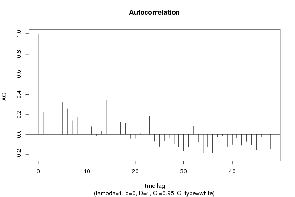
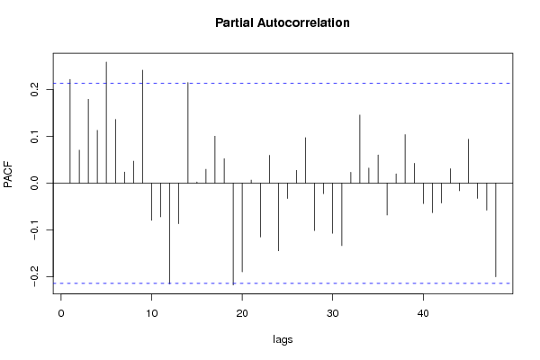
Title produced by software

(Partial) Autocorrelation Function

Date of computation

Mon, 06 Dec 2010 18:25:16 +0000

Cite this page as follows

Statistical Computations at FreeStatistics.org, Office for Research Development and Education, URL https://freestatistics.org/blog/index.php?v=date/2010/Dec/06/t12916598129ekleiuadujgerm.htm/, Retrieved Sun, 28 Apr 2024 19:06:20 +0000

Statistical Computations at FreeStatistics.org, Office for Research Development and Education, URL https://freestatistics.org/blog/index.php?pk=105773, Retrieved Sun, 28 Apr 2024 19:06:20 +0000

QR Codes:

Paste this QR Code to cite your computation.

Original text written by user:

IsPrivate?

No (this computation is public)

User-defined keywords

Estimated Impact

145

Family? (F = Feedback message, R = changed R code, M = changed R Module, P = changed Parameters, D = changed Data)

-     [Univariate Explorative Data Analysis] [Run Sequence gebo...] [2008-12-12 13:32:37] [76963dc1903f0f612b6153510a3818cf]
- R  D  [Univariate Explorative Data Analysis] [Run Sequence gebo...] [2008-12-17 12:14:40] [76963dc1903f0f612b6153510a3818cf]
-         [Univariate Explorative Data Analysis] [Run Sequence Plot...] [2008-12-22 18:19:51] [1ce0d16c8f4225c977b42c8fa93bc163]
- RMP       [Univariate Data Series] [Identifying Integ...] [2009-11-22 12:08:06] [b98453cac15ba1066b407e146608df68]
- RMP         [Variance Reduction Matrix] [Births] [2010-11-29 09:39:41] [b98453cac15ba1066b407e146608df68]
- RMPD          [(Partial) Autocorrelation Function] [seizoenaal diff g...] [2010-12-03 12:03:37] [4eaa304e6a28c475ba490fccf4c01ad3]
- R               [(Partial) Autocorrelation Function] [acf geboortes] [2010-12-03 12:12:39] [4eaa304e6a28c475ba490fccf4c01ad3]
-                   [(Partial) Autocorrelation Function] [non seasonal diff...] [2010-12-03 12:14:02] [4eaa304e6a28c475ba490fccf4c01ad3]
-                     [(Partial) Autocorrelation Function] [seasonal diff geb...] [2010-12-03 12:15:13] [4eaa304e6a28c475ba490fccf4c01ad3]
-   P                     [(Partial) Autocorrelation Function] [seas diff geboortes] [2010-12-06 18:25:16] [e926a978b40506c05812140b9c5157ab] [Current]

Feedback Forum

Post a new message

Dataseries X:

Download CSV

Histogram

Boxplots

Summary of computational transaction
Raw Input	view raw input (R code)
Raw Output	view raw output of R engine
Computing time	1 seconds
R Server	'Gwilym Jenkins' @ 72.249.127.135

\begin{tabular}{lllllllll}
\hline
Summary of computational transaction \tabularnewline
Raw Input & view raw input (R code)  \tabularnewline
Raw Output & view raw output of R engine  \tabularnewline
Computing time & 1 seconds \tabularnewline
R Server & 'Gwilym Jenkins' @ 72.249.127.135 \tabularnewline
\hline
\end{tabular}
%Source: https://freestatistics.org/blog/index.php?pk=105773&T=0

[TABLE]
[ROW][C]Summary of computational transaction[/C][/ROW]
[ROW][C]Raw Input[/C][C]view raw input (R code) [/C][/ROW]
[ROW][C]Raw Output[/C][C]view raw output of R engine [/C][/ROW]
[ROW][C]Computing time[/C][C]1 seconds[/C][/ROW]
[ROW][C]R Server[/C][C]'Gwilym Jenkins' @ 72.249.127.135[/C][/ROW]
[/TABLE]
Source: https://freestatistics.org/blog/index.php?pk=105773&T=0

Globally Unique Identifier (entire table): ba.freestatistics.org/blog/index.php?pk=105773&T=0

As an alternative you can also use a QR Code:

The GUIDs for individual cells are displayed in the table below:

Summary of computational transaction
Raw Input	view raw input (R code)
Raw Output	view raw output of R engine
Computing time	1 seconds
R Server	'Gwilym Jenkins' @ 72.249.127.135

Autocorrelation Function
Time lag k	ACF(k)	T-STAT	P-value
1	0.222208	2.0366	0.022422
2	0.116745	1.07	0.143845
3	0.20959	1.9209	0.029067
4	0.18794	1.7225	0.044329
5	0.316552	2.9012	0.002372
6	0.255511	2.3418	0.010779
7	0.138296	1.2675	0.104238
8	0.171239	1.5694	0.060153
9	0.347708	3.1868	0.00101
10	0.128925	1.1816	0.120347
11	0.079686	0.7303	0.233609
12	-0.017142	-0.1571	0.437769
13	0.03455	0.3167	0.376146
14	0.337045	3.0891	0.001361
15	0.137828	1.2632	0.105004
16	0.056544	0.5182	0.302829
17	0.121729	1.1157	0.133873
18	0.11446	1.049	0.148583
19	-0.040499	-0.3712	0.35572
20	-0.040714	-0.3731	0.354989
21	0.01187	0.1088	0.456813
22	-0.042754	-0.3918	0.348081
23	0.183957	1.686	0.047754
24	-0.068603	-0.6288	0.265609
25	-0.12047	-1.1041	0.136346
26	-0.063995	-0.5865	0.279549
27	-0.032664	-0.2994	0.382699
28	-0.091227	-0.8361	0.202732
29	-0.121044	-1.1094	0.135215
30	-0.161626	-1.4813	0.071131
31	-0.121806	-1.1164	0.133722
32	0.082561	0.7567	0.225678
33	-0.073113	-0.6701	0.252318
34	-0.181409	-1.6626	0.050055
35	-0.121925	-1.1175	0.133491
36	-0.181532	-1.6638	0.049943
37	-0.026024	-0.2385	0.406031
38	-0.012518	-0.1147	0.454467
39	-0.120359	-1.1031	0.136565
40	-0.099807	-0.9147	0.181471
41	-0.033937	-0.311	0.378273
42	-0.107569	-0.9859	0.163509
43	-0.070318	-0.6445	0.260513
44	-0.102411	-0.9386	0.17531
45	-0.150821	-1.3823	0.085273
46	-0.025349	-0.2323	0.408423
47	-0.061573	-0.5643	0.287017
48	-0.144696	-1.3262	0.094191

\begin{tabular}{lllllllll}
\hline
Autocorrelation Function \tabularnewline
Time lag k & ACF(k) & T-STAT & P-value \tabularnewline
1 & 0.222208 & 2.0366 & 0.022422 \tabularnewline
2 & 0.116745 & 1.07 & 0.143845 \tabularnewline
3 & 0.20959 & 1.9209 & 0.029067 \tabularnewline
4 & 0.18794 & 1.7225 & 0.044329 \tabularnewline
5 & 0.316552 & 2.9012 & 0.002372 \tabularnewline
6 & 0.255511 & 2.3418 & 0.010779 \tabularnewline
7 & 0.138296 & 1.2675 & 0.104238 \tabularnewline
8 & 0.171239 & 1.5694 & 0.060153 \tabularnewline
9 & 0.347708 & 3.1868 & 0.00101 \tabularnewline
10 & 0.128925 & 1.1816 & 0.120347 \tabularnewline
11 & 0.079686 & 0.7303 & 0.233609 \tabularnewline
12 & -0.017142 & -0.1571 & 0.437769 \tabularnewline
13 & 0.03455 & 0.3167 & 0.376146 \tabularnewline
14 & 0.337045 & 3.0891 & 0.001361 \tabularnewline
15 & 0.137828 & 1.2632 & 0.105004 \tabularnewline
16 & 0.056544 & 0.5182 & 0.302829 \tabularnewline
17 & 0.121729 & 1.1157 & 0.133873 \tabularnewline
18 & 0.11446 & 1.049 & 0.148583 \tabularnewline
19 & -0.040499 & -0.3712 & 0.35572 \tabularnewline
20 & -0.040714 & -0.3731 & 0.354989 \tabularnewline
21 & 0.01187 & 0.1088 & 0.456813 \tabularnewline
22 & -0.042754 & -0.3918 & 0.348081 \tabularnewline
23 & 0.183957 & 1.686 & 0.047754 \tabularnewline
24 & -0.068603 & -0.6288 & 0.265609 \tabularnewline
25 & -0.12047 & -1.1041 & 0.136346 \tabularnewline
26 & -0.063995 & -0.5865 & 0.279549 \tabularnewline
27 & -0.032664 & -0.2994 & 0.382699 \tabularnewline
28 & -0.091227 & -0.8361 & 0.202732 \tabularnewline
29 & -0.121044 & -1.1094 & 0.135215 \tabularnewline
30 & -0.161626 & -1.4813 & 0.071131 \tabularnewline
31 & -0.121806 & -1.1164 & 0.133722 \tabularnewline
32 & 0.082561 & 0.7567 & 0.225678 \tabularnewline
33 & -0.073113 & -0.6701 & 0.252318 \tabularnewline
34 & -0.181409 & -1.6626 & 0.050055 \tabularnewline
35 & -0.121925 & -1.1175 & 0.133491 \tabularnewline
36 & -0.181532 & -1.6638 & 0.049943 \tabularnewline
37 & -0.026024 & -0.2385 & 0.406031 \tabularnewline
38 & -0.012518 & -0.1147 & 0.454467 \tabularnewline
39 & -0.120359 & -1.1031 & 0.136565 \tabularnewline
40 & -0.099807 & -0.9147 & 0.181471 \tabularnewline
41 & -0.033937 & -0.311 & 0.378273 \tabularnewline
42 & -0.107569 & -0.9859 & 0.163509 \tabularnewline
43 & -0.070318 & -0.6445 & 0.260513 \tabularnewline
44 & -0.102411 & -0.9386 & 0.17531 \tabularnewline
45 & -0.150821 & -1.3823 & 0.085273 \tabularnewline
46 & -0.025349 & -0.2323 & 0.408423 \tabularnewline
47 & -0.061573 & -0.5643 & 0.287017 \tabularnewline
48 & -0.144696 & -1.3262 & 0.094191 \tabularnewline
\hline
\end{tabular}
%Source: https://freestatistics.org/blog/index.php?pk=105773&T=1

[TABLE]
[ROW][C]Autocorrelation Function[/C][/ROW]
[ROW][C]Time lag k[/C][C]ACF(k)[/C][C]T-STAT[/C][C]P-value[/C][/ROW]
[ROW][C]1[/C][C]0.222208[/C][C]2.0366[/C][C]0.022422[/C][/ROW]
[ROW][C]2[/C][C]0.116745[/C][C]1.07[/C][C]0.143845[/C][/ROW]
[ROW][C]3[/C][C]0.20959[/C][C]1.9209[/C][C]0.029067[/C][/ROW]
[ROW][C]4[/C][C]0.18794[/C][C]1.7225[/C][C]0.044329[/C][/ROW]
[ROW][C]5[/C][C]0.316552[/C][C]2.9012[/C][C]0.002372[/C][/ROW]
[ROW][C]6[/C][C]0.255511[/C][C]2.3418[/C][C]0.010779[/C][/ROW]
[ROW][C]7[/C][C]0.138296[/C][C]1.2675[/C][C]0.104238[/C][/ROW]
[ROW][C]8[/C][C]0.171239[/C][C]1.5694[/C][C]0.060153[/C][/ROW]
[ROW][C]9[/C][C]0.347708[/C][C]3.1868[/C][C]0.00101[/C][/ROW]
[ROW][C]10[/C][C]0.128925[/C][C]1.1816[/C][C]0.120347[/C][/ROW]
[ROW][C]11[/C][C]0.079686[/C][C]0.7303[/C][C]0.233609[/C][/ROW]
[ROW][C]12[/C][C]-0.017142[/C][C]-0.1571[/C][C]0.437769[/C][/ROW]
[ROW][C]13[/C][C]0.03455[/C][C]0.3167[/C][C]0.376146[/C][/ROW]
[ROW][C]14[/C][C]0.337045[/C][C]3.0891[/C][C]0.001361[/C][/ROW]
[ROW][C]15[/C][C]0.137828[/C][C]1.2632[/C][C]0.105004[/C][/ROW]
[ROW][C]16[/C][C]0.056544[/C][C]0.5182[/C][C]0.302829[/C][/ROW]
[ROW][C]17[/C][C]0.121729[/C][C]1.1157[/C][C]0.133873[/C][/ROW]
[ROW][C]18[/C][C]0.11446[/C][C]1.049[/C][C]0.148583[/C][/ROW]
[ROW][C]19[/C][C]-0.040499[/C][C]-0.3712[/C][C]0.35572[/C][/ROW]
[ROW][C]20[/C][C]-0.040714[/C][C]-0.3731[/C][C]0.354989[/C][/ROW]
[ROW][C]21[/C][C]0.01187[/C][C]0.1088[/C][C]0.456813[/C][/ROW]
[ROW][C]22[/C][C]-0.042754[/C][C]-0.3918[/C][C]0.348081[/C][/ROW]
[ROW][C]23[/C][C]0.183957[/C][C]1.686[/C][C]0.047754[/C][/ROW]
[ROW][C]24[/C][C]-0.068603[/C][C]-0.6288[/C][C]0.265609[/C][/ROW]
[ROW][C]25[/C][C]-0.12047[/C][C]-1.1041[/C][C]0.136346[/C][/ROW]
[ROW][C]26[/C][C]-0.063995[/C][C]-0.5865[/C][C]0.279549[/C][/ROW]
[ROW][C]27[/C][C]-0.032664[/C][C]-0.2994[/C][C]0.382699[/C][/ROW]
[ROW][C]28[/C][C]-0.091227[/C][C]-0.8361[/C][C]0.202732[/C][/ROW]
[ROW][C]29[/C][C]-0.121044[/C][C]-1.1094[/C][C]0.135215[/C][/ROW]
[ROW][C]30[/C][C]-0.161626[/C][C]-1.4813[/C][C]0.071131[/C][/ROW]
[ROW][C]31[/C][C]-0.121806[/C][C]-1.1164[/C][C]0.133722[/C][/ROW]
[ROW][C]32[/C][C]0.082561[/C][C]0.7567[/C][C]0.225678[/C][/ROW]
[ROW][C]33[/C][C]-0.073113[/C][C]-0.6701[/C][C]0.252318[/C][/ROW]
[ROW][C]34[/C][C]-0.181409[/C][C]-1.6626[/C][C]0.050055[/C][/ROW]
[ROW][C]35[/C][C]-0.121925[/C][C]-1.1175[/C][C]0.133491[/C][/ROW]
[ROW][C]36[/C][C]-0.181532[/C][C]-1.6638[/C][C]0.049943[/C][/ROW]
[ROW][C]37[/C][C]-0.026024[/C][C]-0.2385[/C][C]0.406031[/C][/ROW]
[ROW][C]38[/C][C]-0.012518[/C][C]-0.1147[/C][C]0.454467[/C][/ROW]
[ROW][C]39[/C][C]-0.120359[/C][C]-1.1031[/C][C]0.136565[/C][/ROW]
[ROW][C]40[/C][C]-0.099807[/C][C]-0.9147[/C][C]0.181471[/C][/ROW]
[ROW][C]41[/C][C]-0.033937[/C][C]-0.311[/C][C]0.378273[/C][/ROW]
[ROW][C]42[/C][C]-0.107569[/C][C]-0.9859[/C][C]0.163509[/C][/ROW]
[ROW][C]43[/C][C]-0.070318[/C][C]-0.6445[/C][C]0.260513[/C][/ROW]
[ROW][C]44[/C][C]-0.102411[/C][C]-0.9386[/C][C]0.17531[/C][/ROW]
[ROW][C]45[/C][C]-0.150821[/C][C]-1.3823[/C][C]0.085273[/C][/ROW]
[ROW][C]46[/C][C]-0.025349[/C][C]-0.2323[/C][C]0.408423[/C][/ROW]
[ROW][C]47[/C][C]-0.061573[/C][C]-0.5643[/C][C]0.287017[/C][/ROW]
[ROW][C]48[/C][C]-0.144696[/C][C]-1.3262[/C][C]0.094191[/C][/ROW]
[/TABLE]
Source: https://freestatistics.org/blog/index.php?pk=105773&T=1

Globally Unique Identifier (entire table): ba.freestatistics.org/blog/index.php?pk=105773&T=1

As an alternative you can also use a QR Code:

The GUIDs for individual cells are displayed in the table below:

Autocorrelation Function
Time lag k	ACF(k)	T-STAT	P-value
1	0.222208	2.0366	0.022422
2	0.116745	1.07	0.143845
3	0.20959	1.9209	0.029067
4	0.18794	1.7225	0.044329
5	0.316552	2.9012	0.002372
6	0.255511	2.3418	0.010779
7	0.138296	1.2675	0.104238
8	0.171239	1.5694	0.060153
9	0.347708	3.1868	0.00101
10	0.128925	1.1816	0.120347
11	0.079686	0.7303	0.233609
12	-0.017142	-0.1571	0.437769
13	0.03455	0.3167	0.376146
14	0.337045	3.0891	0.001361
15	0.137828	1.2632	0.105004
16	0.056544	0.5182	0.302829
17	0.121729	1.1157	0.133873
18	0.11446	1.049	0.148583
19	-0.040499	-0.3712	0.35572
20	-0.040714	-0.3731	0.354989
21	0.01187	0.1088	0.456813
22	-0.042754	-0.3918	0.348081
23	0.183957	1.686	0.047754
24	-0.068603	-0.6288	0.265609
25	-0.12047	-1.1041	0.136346
26	-0.063995	-0.5865	0.279549
27	-0.032664	-0.2994	0.382699
28	-0.091227	-0.8361	0.202732
29	-0.121044	-1.1094	0.135215
30	-0.161626	-1.4813	0.071131
31	-0.121806	-1.1164	0.133722
32	0.082561	0.7567	0.225678
33	-0.073113	-0.6701	0.252318
34	-0.181409	-1.6626	0.050055
35	-0.121925	-1.1175	0.133491
36	-0.181532	-1.6638	0.049943
37	-0.026024	-0.2385	0.406031
38	-0.012518	-0.1147	0.454467
39	-0.120359	-1.1031	0.136565
40	-0.099807	-0.9147	0.181471
41	-0.033937	-0.311	0.378273
42	-0.107569	-0.9859	0.163509
43	-0.070318	-0.6445	0.260513
44	-0.102411	-0.9386	0.17531
45	-0.150821	-1.3823	0.085273
46	-0.025349	-0.2323	0.408423
47	-0.061573	-0.5643	0.287017
48	-0.144696	-1.3262	0.094191

Partial Autocorrelation Function
Time lag k	PACF(k)	T-STAT	P-value
1	0.222208	2.0366	0.022422
2	0.070868	0.6495	0.258888
3	0.179457	1.6448	0.051879
4	0.113076	1.0364	0.151504
5	0.259103	2.3747	0.00992
6	0.136408	1.2502	0.10735
7	0.023812	0.2182	0.413885
8	0.047307	0.4336	0.332856
9	0.241832	2.2164	0.014683
10	-0.079304	-0.7268	0.234673
11	-0.071824	-0.6583	0.256079
12	-0.215246	-1.9728	0.025906
13	-0.086512	-0.7929	0.215035
14	0.215465	1.9748	0.02579
15	0.002734	0.0251	0.490035
16	0.029958	0.2746	0.39216
17	0.100709	0.923	0.179321
18	0.052629	0.4824	0.315404
19	-0.217464	-1.9931	0.024749
20	-0.189514	-1.7369	0.043033
21	0.006968	0.0639	0.474616
22	-0.114736	-1.0516	0.148006
23	0.05977	0.5478	0.292641
24	-0.144347	-1.323	0.094719
25	-0.032607	-0.2988	0.382897
26	0.027468	0.2517	0.400926
27	0.097418	0.8929	0.187243
28	-0.101231	-0.9278	0.178085
29	-0.022237	-0.2038	0.419499
30	-0.107016	-0.9808	0.16475
31	-0.133406	-1.2227	0.112433
32	0.023346	0.214	0.415545
33	0.145879	1.337	0.092416
34	0.032503	0.2979	0.383258
35	0.060373	0.5533	0.290754
36	-0.067987	-0.6231	0.26745
37	0.020012	0.1834	0.427457
38	0.103887	0.9521	0.171878
39	0.042625	0.3907	0.348516
40	-0.043465	-0.3984	0.345686
41	-0.062935	-0.5768	0.282807
42	-0.042214	-0.3869	0.349905
43	0.031178	0.2857	0.387887
44	-0.015911	-0.1458	0.442203
45	0.094154	0.8629	0.195315
46	-0.032343	-0.2964	0.383816
47	-0.057648	-0.5284	0.299323
48	-0.19991	-1.8322	0.035232

\begin{tabular}{lllllllll}
\hline
Partial Autocorrelation Function \tabularnewline
Time lag k & PACF(k) & T-STAT & P-value \tabularnewline
1 & 0.222208 & 2.0366 & 0.022422 \tabularnewline
2 & 0.070868 & 0.6495 & 0.258888 \tabularnewline
3 & 0.179457 & 1.6448 & 0.051879 \tabularnewline
4 & 0.113076 & 1.0364 & 0.151504 \tabularnewline
5 & 0.259103 & 2.3747 & 0.00992 \tabularnewline
6 & 0.136408 & 1.2502 & 0.10735 \tabularnewline
7 & 0.023812 & 0.2182 & 0.413885 \tabularnewline
8 & 0.047307 & 0.4336 & 0.332856 \tabularnewline
9 & 0.241832 & 2.2164 & 0.014683 \tabularnewline
10 & -0.079304 & -0.7268 & 0.234673 \tabularnewline
11 & -0.071824 & -0.6583 & 0.256079 \tabularnewline
12 & -0.215246 & -1.9728 & 0.025906 \tabularnewline
13 & -0.086512 & -0.7929 & 0.215035 \tabularnewline
14 & 0.215465 & 1.9748 & 0.02579 \tabularnewline
15 & 0.002734 & 0.0251 & 0.490035 \tabularnewline
16 & 0.029958 & 0.2746 & 0.39216 \tabularnewline
17 & 0.100709 & 0.923 & 0.179321 \tabularnewline
18 & 0.052629 & 0.4824 & 0.315404 \tabularnewline
19 & -0.217464 & -1.9931 & 0.024749 \tabularnewline
20 & -0.189514 & -1.7369 & 0.043033 \tabularnewline
21 & 0.006968 & 0.0639 & 0.474616 \tabularnewline
22 & -0.114736 & -1.0516 & 0.148006 \tabularnewline
23 & 0.05977 & 0.5478 & 0.292641 \tabularnewline
24 & -0.144347 & -1.323 & 0.094719 \tabularnewline
25 & -0.032607 & -0.2988 & 0.382897 \tabularnewline
26 & 0.027468 & 0.2517 & 0.400926 \tabularnewline
27 & 0.097418 & 0.8929 & 0.187243 \tabularnewline
28 & -0.101231 & -0.9278 & 0.178085 \tabularnewline
29 & -0.022237 & -0.2038 & 0.419499 \tabularnewline
30 & -0.107016 & -0.9808 & 0.16475 \tabularnewline
31 & -0.133406 & -1.2227 & 0.112433 \tabularnewline
32 & 0.023346 & 0.214 & 0.415545 \tabularnewline
33 & 0.145879 & 1.337 & 0.092416 \tabularnewline
34 & 0.032503 & 0.2979 & 0.383258 \tabularnewline
35 & 0.060373 & 0.5533 & 0.290754 \tabularnewline
36 & -0.067987 & -0.6231 & 0.26745 \tabularnewline
37 & 0.020012 & 0.1834 & 0.427457 \tabularnewline
38 & 0.103887 & 0.9521 & 0.171878 \tabularnewline
39 & 0.042625 & 0.3907 & 0.348516 \tabularnewline
40 & -0.043465 & -0.3984 & 0.345686 \tabularnewline
41 & -0.062935 & -0.5768 & 0.282807 \tabularnewline
42 & -0.042214 & -0.3869 & 0.349905 \tabularnewline
43 & 0.031178 & 0.2857 & 0.387887 \tabularnewline
44 & -0.015911 & -0.1458 & 0.442203 \tabularnewline
45 & 0.094154 & 0.8629 & 0.195315 \tabularnewline
46 & -0.032343 & -0.2964 & 0.383816 \tabularnewline
47 & -0.057648 & -0.5284 & 0.299323 \tabularnewline
48 & -0.19991 & -1.8322 & 0.035232 \tabularnewline
\hline
\end{tabular}
%Source: https://freestatistics.org/blog/index.php?pk=105773&T=2

[TABLE]
[ROW][C]Partial Autocorrelation Function[/C][/ROW]
[ROW][C]Time lag k[/C][C]PACF(k)[/C][C]T-STAT[/C][C]P-value[/C][/ROW]
[ROW][C]1[/C][C]0.222208[/C][C]2.0366[/C][C]0.022422[/C][/ROW]
[ROW][C]2[/C][C]0.070868[/C][C]0.6495[/C][C]0.258888[/C][/ROW]
[ROW][C]3[/C][C]0.179457[/C][C]1.6448[/C][C]0.051879[/C][/ROW]
[ROW][C]4[/C][C]0.113076[/C][C]1.0364[/C][C]0.151504[/C][/ROW]
[ROW][C]5[/C][C]0.259103[/C][C]2.3747[/C][C]0.00992[/C][/ROW]
[ROW][C]6[/C][C]0.136408[/C][C]1.2502[/C][C]0.10735[/C][/ROW]
[ROW][C]7[/C][C]0.023812[/C][C]0.2182[/C][C]0.413885[/C][/ROW]
[ROW][C]8[/C][C]0.047307[/C][C]0.4336[/C][C]0.332856[/C][/ROW]
[ROW][C]9[/C][C]0.241832[/C][C]2.2164[/C][C]0.014683[/C][/ROW]
[ROW][C]10[/C][C]-0.079304[/C][C]-0.7268[/C][C]0.234673[/C][/ROW]
[ROW][C]11[/C][C]-0.071824[/C][C]-0.6583[/C][C]0.256079[/C][/ROW]
[ROW][C]12[/C][C]-0.215246[/C][C]-1.9728[/C][C]0.025906[/C][/ROW]
[ROW][C]13[/C][C]-0.086512[/C][C]-0.7929[/C][C]0.215035[/C][/ROW]
[ROW][C]14[/C][C]0.215465[/C][C]1.9748[/C][C]0.02579[/C][/ROW]
[ROW][C]15[/C][C]0.002734[/C][C]0.0251[/C][C]0.490035[/C][/ROW]
[ROW][C]16[/C][C]0.029958[/C][C]0.2746[/C][C]0.39216[/C][/ROW]
[ROW][C]17[/C][C]0.100709[/C][C]0.923[/C][C]0.179321[/C][/ROW]
[ROW][C]18[/C][C]0.052629[/C][C]0.4824[/C][C]0.315404[/C][/ROW]
[ROW][C]19[/C][C]-0.217464[/C][C]-1.9931[/C][C]0.024749[/C][/ROW]
[ROW][C]20[/C][C]-0.189514[/C][C]-1.7369[/C][C]0.043033[/C][/ROW]
[ROW][C]21[/C][C]0.006968[/C][C]0.0639[/C][C]0.474616[/C][/ROW]
[ROW][C]22[/C][C]-0.114736[/C][C]-1.0516[/C][C]0.148006[/C][/ROW]
[ROW][C]23[/C][C]0.05977[/C][C]0.5478[/C][C]0.292641[/C][/ROW]
[ROW][C]24[/C][C]-0.144347[/C][C]-1.323[/C][C]0.094719[/C][/ROW]
[ROW][C]25[/C][C]-0.032607[/C][C]-0.2988[/C][C]0.382897[/C][/ROW]
[ROW][C]26[/C][C]0.027468[/C][C]0.2517[/C][C]0.400926[/C][/ROW]
[ROW][C]27[/C][C]0.097418[/C][C]0.8929[/C][C]0.187243[/C][/ROW]
[ROW][C]28[/C][C]-0.101231[/C][C]-0.9278[/C][C]0.178085[/C][/ROW]
[ROW][C]29[/C][C]-0.022237[/C][C]-0.2038[/C][C]0.419499[/C][/ROW]
[ROW][C]30[/C][C]-0.107016[/C][C]-0.9808[/C][C]0.16475[/C][/ROW]
[ROW][C]31[/C][C]-0.133406[/C][C]-1.2227[/C][C]0.112433[/C][/ROW]
[ROW][C]32[/C][C]0.023346[/C][C]0.214[/C][C]0.415545[/C][/ROW]
[ROW][C]33[/C][C]0.145879[/C][C]1.337[/C][C]0.092416[/C][/ROW]
[ROW][C]34[/C][C]0.032503[/C][C]0.2979[/C][C]0.383258[/C][/ROW]
[ROW][C]35[/C][C]0.060373[/C][C]0.5533[/C][C]0.290754[/C][/ROW]
[ROW][C]36[/C][C]-0.067987[/C][C]-0.6231[/C][C]0.26745[/C][/ROW]
[ROW][C]37[/C][C]0.020012[/C][C]0.1834[/C][C]0.427457[/C][/ROW]
[ROW][C]38[/C][C]0.103887[/C][C]0.9521[/C][C]0.171878[/C][/ROW]
[ROW][C]39[/C][C]0.042625[/C][C]0.3907[/C][C]0.348516[/C][/ROW]
[ROW][C]40[/C][C]-0.043465[/C][C]-0.3984[/C][C]0.345686[/C][/ROW]
[ROW][C]41[/C][C]-0.062935[/C][C]-0.5768[/C][C]0.282807[/C][/ROW]
[ROW][C]42[/C][C]-0.042214[/C][C]-0.3869[/C][C]0.349905[/C][/ROW]
[ROW][C]43[/C][C]0.031178[/C][C]0.2857[/C][C]0.387887[/C][/ROW]
[ROW][C]44[/C][C]-0.015911[/C][C]-0.1458[/C][C]0.442203[/C][/ROW]
[ROW][C]45[/C][C]0.094154[/C][C]0.8629[/C][C]0.195315[/C][/ROW]
[ROW][C]46[/C][C]-0.032343[/C][C]-0.2964[/C][C]0.383816[/C][/ROW]
[ROW][C]47[/C][C]-0.057648[/C][C]-0.5284[/C][C]0.299323[/C][/ROW]
[ROW][C]48[/C][C]-0.19991[/C][C]-1.8322[/C][C]0.035232[/C][/ROW]
[/TABLE]
Source: https://freestatistics.org/blog/index.php?pk=105773&T=2

Globally Unique Identifier (entire table): ba.freestatistics.org/blog/index.php?pk=105773&T=2

As an alternative you can also use a QR Code:

The GUIDs for individual cells are displayed in the table below:

Partial Autocorrelation Function
Time lag k	PACF(k)	T-STAT	P-value
1	0.222208	2.0366	0.022422
2	0.070868	0.6495	0.258888
3	0.179457	1.6448	0.051879
4	0.113076	1.0364	0.151504
5	0.259103	2.3747	0.00992
6	0.136408	1.2502	0.10735
7	0.023812	0.2182	0.413885
8	0.047307	0.4336	0.332856
9	0.241832	2.2164	0.014683
10	-0.079304	-0.7268	0.234673
11	-0.071824	-0.6583	0.256079
12	-0.215246	-1.9728	0.025906
13	-0.086512	-0.7929	0.215035
14	0.215465	1.9748	0.02579
15	0.002734	0.0251	0.490035
16	0.029958	0.2746	0.39216
17	0.100709	0.923	0.179321
18	0.052629	0.4824	0.315404
19	-0.217464	-1.9931	0.024749
20	-0.189514	-1.7369	0.043033
21	0.006968	0.0639	0.474616
22	-0.114736	-1.0516	0.148006
23	0.05977	0.5478	0.292641
24	-0.144347	-1.323	0.094719
25	-0.032607	-0.2988	0.382897
26	0.027468	0.2517	0.400926
27	0.097418	0.8929	0.187243
28	-0.101231	-0.9278	0.178085
29	-0.022237	-0.2038	0.419499
30	-0.107016	-0.9808	0.16475
31	-0.133406	-1.2227	0.112433
32	0.023346	0.214	0.415545
33	0.145879	1.337	0.092416
34	0.032503	0.2979	0.383258
35	0.060373	0.5533	0.290754
36	-0.067987	-0.6231	0.26745
37	0.020012	0.1834	0.427457
38	0.103887	0.9521	0.171878
39	0.042625	0.3907	0.348516
40	-0.043465	-0.3984	0.345686
41	-0.062935	-0.5768	0.282807
42	-0.042214	-0.3869	0.349905
43	0.031178	0.2857	0.387887
44	-0.015911	-0.1458	0.442203
45	0.094154	0.8629	0.195315
46	-0.032343	-0.2964	0.383816
47	-0.057648	-0.5284	0.299323
48	-0.19991	-1.8322	0.035232

Figure 1

PNG link

Postscript link

PDF link

Figure 2

PNG link

Postscript link

PDF link

Parameters (Session):

par1 = 48 ; par2 = 1 ; par3 = 0 ; par4 = 1 ; par5 = 12 ; par6 = White Noise ; par7 = 0.95 ;

Parameters (R input):

par1 = 48 ; par2 = 1 ; par3 = 0 ; par4 = 1 ; par5 = 12 ; par6 = White Noise ; par7 = 0.95 ;

R code (references can be found in the software module):

if (par1 == 'Default') {
par1 = 10*log10(length(x))
} else {
par1 <- as.numeric(par1)
}
par2 <- as.numeric(par2)
par3 <- as.numeric(par3)
par4 <- as.numeric(par4)
par5 <- as.numeric(par5)
if (par6 == 'White Noise') par6 <- 'white' else par6 <- 'ma'
par7 <- as.numeric(par7)
if (par2 == 0) {
x <- log(x)
} else {
x <- (x ^ par2 - 1) / par2
}
if (par3 > 0) x <- diff(x,lag=1,difference=par3)
if (par4 > 0) x <- diff(x,lag=par5,difference=par4)
bitmap(file='pic1.png')
racf <- acf(x, par1, main='Autocorrelation', xlab='time lag', ylab='ACF', ci.type=par6, ci=par7, sub=paste('(lambda=',par2,', d=',par3,', D=',par4,', CI=', par7, ', CI type=',par6,')',sep=''))
dev.off()
bitmap(file='pic2.png')
rpacf <- pacf(x,par1,main='Partial Autocorrelation',xlab='lags',ylab='PACF')
dev.off()
(myacf <- c(racf$acf))
(mypacf <- c(rpacf$acf))
lengthx <- length(x)
sqrtn <- sqrt(lengthx)
load(file='createtable')
a<-table.start()
a<-table.row.start(a)
a<-table.element(a,'Autocorrelation Function',4,TRUE)
a<-table.row.end(a)
a<-table.row.start(a)
a<-table.element(a,'Time lag k',header=TRUE)
a<-table.element(a,hyperlink('basics.htm','ACF(k)','click here for more information about the Autocorrelation Function'),header=TRUE)
a<-table.element(a,'T-STAT',header=TRUE)
a<-table.element(a,'P-value',header=TRUE)
a<-table.row.end(a)
for (i in 2:(par1+1)) {
a<-table.row.start(a)
a<-table.element(a,i-1,header=TRUE)
a<-table.element(a,round(myacf[i],6))
mytstat <- myacf[i]*sqrtn
a<-table.element(a,round(mytstat,4))
a<-table.element(a,round(1-pt(abs(mytstat),lengthx),6))
a<-table.row.end(a)
}
a<-table.end(a)
table.save(a,file='mytable.tab')
a<-table.start()
a<-table.row.start(a)
a<-table.element(a,'Partial Autocorrelation Function',4,TRUE)
a<-table.row.end(a)
a<-table.row.start(a)
a<-table.element(a,'Time lag k',header=TRUE)
a<-table.element(a,hyperlink('basics.htm','PACF(k)','click here for more information about the Partial Autocorrelation Function'),header=TRUE)
a<-table.element(a,'T-STAT',header=TRUE)
a<-table.element(a,'P-value',header=TRUE)
a<-table.row.end(a)
for (i in 1:par1) {
a<-table.row.start(a)
a<-table.element(a,i,header=TRUE)
a<-table.element(a,round(mypacf[i],6))
mytstat <- mypacf[i]*sqrtn
a<-table.element(a,round(mytstat,4))
a<-table.element(a,round(1-pt(abs(mytstat),lengthx),6))
a<-table.row.end(a)
}
a<-table.end(a)
table.save(a,file='mytable1.tab')

Free Statistics

Description of Statistical Computation

Tree of Dependent Computations

Dataset

Tables (Output of Computation)

Figures (Output of Computation)

Input Parameters & R Code