| Multiple Linear Regression - Estimated Regression Equation |
| BEL_20[t] = + 392.801288384327 + 0.0390117340790035Nikkei[t] + 0.103211876652727DJ_Indust[t] -0.00376644874838964Goudprijs[t] -14.5419039745120Conjunct_Seizoenzuiver[t] + 2.61444593841881Cons_vertrouw[t] -9.80081512339516Alg_consumptie_index_BE[t] + 17.3973640331083Gem_rente_kasbon_1j[t] -57.0314960208367M1[t] -24.2910866948577M2[t] -68.8468361794204M3[t] -177.959481264132M4[t] -157.806908916677M5[t] -123.370114378759M6[t] -104.388896451179M7[t] -67.7757332668275M8[t] -73.258344759955M9[t] -80.9274531305978M10[t] -30.5574705031455M11[t] + 46.2909033428714t + e[t] |
| Multiple Linear Regression - Ordinary Least Squares | |||||
| Variable | Parameter | S.D. | T-STAT H0: parameter = 0 | 2-tail p-value | 1-tail p-value |
| (Intercept) | 392.801288384327 | 451.46816 | 0.8701 | 0.390959 | 0.195479 |
| Nikkei | 0.0390117340790035 | 0.025683 | 1.519 | 0.138907 | 0.069454 |
| DJ_Indust | 0.103211876652727 | 0.040347 | 2.5581 | 0.015631 | 0.007816 |
| Goudprijs | -0.00376644874838964 | 0.029935 | -0.1258 | 0.900686 | 0.450343 |
| Conjunct_Seizoenzuiver | -14.5419039745120 | 3.735235 | -3.8932 | 0.000491 | 0.000246 |
| Cons_vertrouw | 2.61444593841881 | 4.160018 | 0.6285 | 0.5343 | 0.26715 |
| Alg_consumptie_index_BE | -9.80081512339516 | 30.457203 | -0.3218 | 0.749772 | 0.374886 |
| Gem_rente_kasbon_1j | 17.3973640331083 | 56.096561 | 0.3101 | 0.758536 | 0.379268 |
| M1 | -57.0314960208367 | 51.127239 | -1.1155 | 0.273217 | 0.136608 |
| M2 | -24.2910866948577 | 49.266601 | -0.4931 | 0.625449 | 0.312725 |
| M3 | -68.8468361794204 | 50.988367 | -1.3502 | 0.186713 | 0.093357 |
| M4 | -177.959481264132 | 52.400296 | -3.3962 | 0.00189 | 0.000945 |
| M5 | -157.806908916677 | 54.558946 | -2.8924 | 0.006933 | 0.003466 |
| M6 | -123.370114378759 | 53.068577 | -2.3247 | 0.026808 | 0.013404 |
| M7 | -104.388896451179 | 53.577203 | -1.9484 | 0.060471 | 0.030236 |
| M8 | -67.7757332668275 | 56.453558 | -1.2006 | 0.239017 | 0.119508 |
| M9 | -73.258344759955 | 53.008284 | -1.382 | 0.176845 | 0.088422 |
| M10 | -80.9274531305978 | 53.817464 | -1.5037 | 0.142769 | 0.071384 |
| M11 | -30.5574705031455 | 50.772152 | -0.6019 | 0.551647 | 0.275824 |
| t | 46.2909033428714 | 3.413504 | 13.5611 | 0 | 0 |
| Multiple Linear Regression - Regression Statistics | |
| Multiple R | 0.99781758983681 |
| R-squared | 0.99563994258774 |
| Adjusted R-squared | 0.992967649335064 |
| F-TEST (value) | 372.57884836959 |
| F-TEST (DF numerator) | 19 |
| F-TEST (DF denominator) | 31 |
| p-value | 0 |
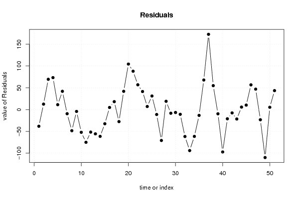
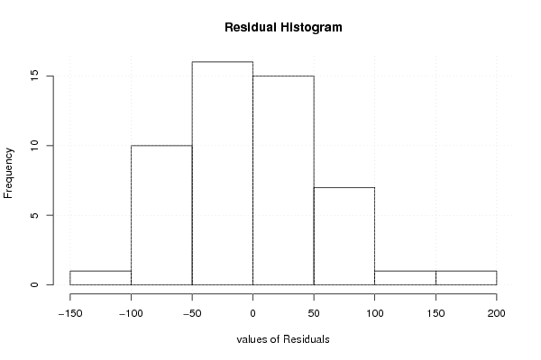
| Multiple Linear Regression - Residual Statistics | |
| Residual Standard Deviation | 70.3151203550974 |
| Sum Squared Residuals | 153270.700667107 |
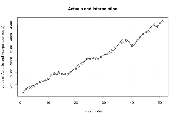
| Multiple Linear Regression - Actuals, Interpolation, and Residuals | |||
| Time or Index | Actuals | Interpolation Forecast | Residuals Prediction Error |
| 1 | 1635.25 | 1673.49292701275 | -38.2429270127463 |
| 2 | 1833.42 | 1820.91087552158 | 12.5091244784202 |
| 3 | 1910.43 | 1840.92816888193 | 69.5018311180717 |
| 4 | 1959.67 | 1886.28759564899 | 73.3824043510058 |
| 5 | 1969.6 | 1958.32963635339 | 11.2703636466069 |
| 6 | 2061.41 | 2019.4711363995 | 41.9388636005008 |
| 7 | 2093.48 | 2102.92006092129 | -9.44006092128817 |
| 8 | 2120.88 | 2169.33253754454 | -48.4525375445359 |
| 9 | 2174.56 | 2178.79200781225 | -4.23200781224703 |
| 10 | 2196.72 | 2248.87077728972 | -52.1507772897242 |
| 11 | 2350.44 | 2425.56981480826 | -75.129814808255 |
| 12 | 2440.25 | 2491.92217616365 | -51.6721761636549 |
| 13 | 2408.64 | 2464.35061615865 | -55.7106161586485 |
| 14 | 2472.81 | 2534.30292101813 | -61.4929210181315 |
| 15 | 2407.6 | 2440.07831424644 | -32.47831424644 |
| 16 | 2454.62 | 2449.7816303697 | 4.83836963030146 |
| 17 | 2448.05 | 2429.84902576323 | 18.2009742367661 |
| 18 | 2497.84 | 2525.41819221783 | -27.5781922178349 |
| 19 | 2645.64 | 2603.70408558155 | 41.9359144184471 |
| 20 | 2756.76 | 2652.21364834295 | 104.546351657051 |
| 21 | 2849.27 | 2761.22337647946 | 88.0466235205374 |
| 22 | 2921.44 | 2864.49720729208 | 56.9427927079155 |
| 23 | 2981.85 | 2940.37821053709 | 41.4717894629134 |
| 24 | 3080.58 | 3073.52065743784 | 7.05934256215633 |
| 25 | 3106.22 | 3075.02316385870 | 31.1968361413031 |
| 26 | 3119.31 | 3130.59273385449 | -11.2827338544854 |
| 27 | 3061.26 | 3132.15080376903 | -70.8908037690295 |
| 28 | 3097.31 | 3078.26377163835 | 19.0462283616461 |
| 29 | 3161.69 | 3170.05199828856 | -8.36199828855813 |
| 30 | 3257.16 | 3263.88514642856 | -6.72514642856179 |
| 31 | 3277.01 | 3287.84604739132 | -10.8360473913194 |
| 32 | 3295.32 | 3357.13947360702 | -61.8194736070175 |
| 33 | 3363.99 | 3458.07551070388 | -94.0855107038814 |
| 34 | 3494.17 | 3555.73819354145 | -61.5681935414468 |
| 35 | 3667.03 | 3680.32954003481 | -13.2995400348056 |
| 36 | 3813.06 | 3745.12903704301 | 67.930962956988 |
| 37 | 3917.96 | 3745.11625910004 | 172.843740899956 |
| 38 | 3895.51 | 3840.5301065119 | 54.9798934880987 |
| 39 | 3801.06 | 3810.70877594373 | -9.64877594372815 |
| 40 | 3570.12 | 3667.38700234295 | -97.2670023429533 |
| 41 | 3701.61 | 3722.71933959481 | -21.1093395948148 |
| 42 | 3862.27 | 3869.90552495410 | -7.63552495410401 |
| 43 | 3970.1 | 3991.75980610584 | -21.6598061058396 |
| 44 | 4138.52 | 4132.7943405055 | 5.72565949450227 |
| 45 | 4199.75 | 4189.47910500441 | 10.2708949955911 |
| 46 | 4290.89 | 4234.11382187674 | 56.7761781232554 |
| 47 | 4443.91 | 4396.95243461985 | 46.9575653801472 |
| 48 | 4502.64 | 4525.95812935549 | -23.3181293554894 |
| 49 | 4356.98 | 4467.06703386986 | -110.087033869865 |
| 50 | 4591.27 | 4585.9833630939 | 5.28663690609805 |
| 51 | 4696.96 | 4653.44393715887 | 43.516062841126 |
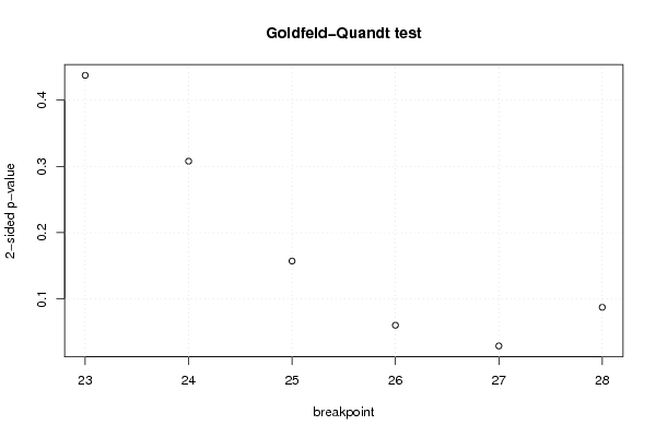
| Goldfeld-Quandt test for Heteroskedasticity | |||
| p-values | Alternative Hypothesis | ||
| breakpoint index | greater | 2-sided | less |
| 23 | 0.781207784446503 | 0.437584431106994 | 0.218792215553497 |
| 24 | 0.84607582312392 | 0.307848353752161 | 0.153924176876080 |
| 25 | 0.921450782707052 | 0.157098434585895 | 0.0785492172929477 |
| 26 | 0.969913392056217 | 0.0601732158875662 | 0.0300866079437831 |
| 27 | 0.985566722698223 | 0.0288665546035542 | 0.0144332773017771 |
| 28 | 0.95638680809909 | 0.08722638380182 | 0.04361319190091 |
| Meta Analysis of Goldfeld-Quandt test for Heteroskedasticity | |||
| Description | # significant tests | % significant tests | OK/NOK |
| 1% type I error level | 0 | 0 | OK |
| 5% type I error level | 1 | 0.166666666666667 | NOK |
| 10% type I error level | 3 | 0.5 | NOK |