Repository of Reproducible Computations

Free Statistics

of Irreproducible Research!

Author's title

Author

*The author of this computation has been verified*

R Software Module

rwasp_autocorrelation.wasp

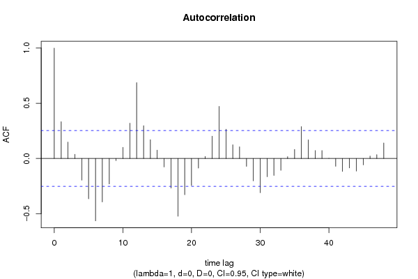
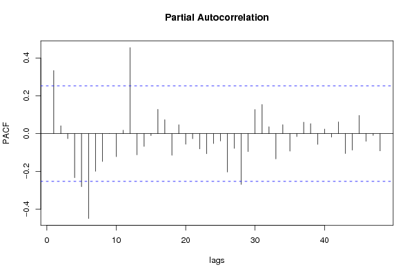
Title produced by software

(Partial) Autocorrelation Function

Date of computation

Fri, 03 Dec 2010 10:48:00 +0000

Cite this page as follows

Statistical Computations at FreeStatistics.org, Office for Research Development and Education, URL https://freestatistics.org/blog/index.php?v=date/2010/Dec/03/t1291373228ieu3vt5vawkdfd1.htm/, Retrieved Tue, 07 May 2024 21:28:41 +0000

Statistical Computations at FreeStatistics.org, Office for Research Development and Education, URL https://freestatistics.org/blog/index.php?pk=104627, Retrieved Tue, 07 May 2024 21:28:41 +0000

QR Codes:

Paste this QR Code to cite your computation.

Original text written by user:

IsPrivate?

No (this computation is public)

User-defined keywords

Estimated Impact

207

Family? (F = Feedback message, R = changed R code, M = changed R Module, P = changed Parameters, D = changed Data)

-     [Univariate Data Series] [data set] [2008-12-01 19:54:57] [b98453cac15ba1066b407e146608df68]
- RMP   [(Partial) Autocorrelation Function] [Unemployment] [2010-11-29 09:05:21] [b98453cac15ba1066b407e146608df68]
-    D    [(Partial) Autocorrelation Function] [Workshop 9] [2010-12-03 10:43:29] [39c51da0be01189e8a44eb69e891b7a1]
-   P         [(Partial) Autocorrelation Function] [Workshop 9] [2010-12-03 10:48:00] [ecfb965f5669057f3ac5b58964283289] [Current]
-   P           [(Partial) Autocorrelation Function] [Workshop 9] [2010-12-03 12:19:31] [39c51da0be01189e8a44eb69e891b7a1] 
-    D            [(Partial) Autocorrelation Function] [Autocorrelation A...] [2010-12-21 12:22:09] [f9eaed74daea918f73b9f505c5b1f19e] 
-   P               [(Partial) Autocorrelation Function] [Autocorrelation A...] [2010-12-21 13:51:25] [f9eaed74daea918f73b9f505c5b1f19e] 
-   P               [(Partial) Autocorrelation Function] [Autocorrelation A...] [2010-12-21 14:56:54] [f9eaed74daea918f73b9f505c5b1f19e] 
-    D          [(Partial) Autocorrelation Function] [Autocorrelation ACF] [2010-12-21 11:32:47] [f9eaed74daea918f73b9f505c5b1f19e] 

Feedback Forum

Post a new message

Dataseries X:

Download CSV

Histogram

Boxplots

Summary of computational transaction
Raw Input	view raw input (R code)
Raw Output	view raw output of R engine
Computing time	2 seconds
R Server	'Sir Ronald Aylmer Fisher' @ 193.190.124.24

\begin{tabular}{lllllllll}
\hline
Summary of computational transaction \tabularnewline
Raw Input & view raw input (R code)  \tabularnewline
Raw Output & view raw output of R engine  \tabularnewline
Computing time & 2 seconds \tabularnewline
R Server & 'Sir Ronald Aylmer Fisher' @ 193.190.124.24 \tabularnewline
\hline
\end{tabular}
%Source: https://freestatistics.org/blog/index.php?pk=104627&T=0

[TABLE]
[ROW][C]Summary of computational transaction[/C][/ROW]
[ROW][C]Raw Input[/C][C]view raw input (R code) [/C][/ROW]
[ROW][C]Raw Output[/C][C]view raw output of R engine [/C][/ROW]
[ROW][C]Computing time[/C][C]2 seconds[/C][/ROW]
[ROW][C]R Server[/C][C]'Sir Ronald Aylmer Fisher' @ 193.190.124.24[/C][/ROW]
[/TABLE]
Source: https://freestatistics.org/blog/index.php?pk=104627&T=0

Globally Unique Identifier (entire table): ba.freestatistics.org/blog/index.php?pk=104627&T=0

As an alternative you can also use a QR Code:

The GUIDs for individual cells are displayed in the table below:

Summary of computational transaction
Raw Input	view raw input (R code)
Raw Output	view raw output of R engine
Computing time	2 seconds
R Server	'Sir Ronald Aylmer Fisher' @ 193.190.124.24

Autocorrelation Function
Time lag k	ACF(k)	T-STAT	P-value
1	0.33367	2.5846	0.0061
2	0.148125	1.1474	0.127891
3	0.037858	0.2932	0.385172
4	-0.195877	-1.5173	0.067226
5	-0.365484	-2.831	0.003152
6	-0.565263	-4.3785	2.4e-05
7	-0.393652	-3.0492	0.001706
8	-0.231438	-1.7927	0.03903
9	-0.019435	-0.1505	0.44042
10	0.101469	0.786	0.217488
11	0.319608	2.4757	0.008069
12	0.686578	5.3182	1e-06
13	0.297152	2.3017	0.012419
14	0.169604	1.3137	0.096967
15	0.075551	0.5852	0.280298
16	-0.077209	-0.5981	0.276026
17	-0.268161	-2.0772	0.021038
18	-0.523486	-4.0549	7.3e-05
19	-0.328207	-2.5423	0.006806
20	-0.245427	-1.9011	0.03105
21	-0.087054	-0.6743	0.25135
22	0.018129	0.1404	0.444397
23	0.201756	1.5628	0.06168
24	0.472728	3.6617	0.000266
25	0.265062	2.0532	0.022212
26	0.123975	0.9603	0.170378
27	0.106196	0.8226	0.207
28	-0.07187	-0.5567	0.289901
29	-0.202442	-1.5681	0.061057
30	-0.310603	-2.4059	0.009615
31	-0.165687	-1.2834	0.102142
32	-0.153603	-1.1898	0.119405
33	-0.107234	-0.8306	0.204738
34	0.016291	0.1262	0.450001
35	0.082063	0.6357	0.263708
36	0.289209	2.2402	0.014397
37	0.169202	1.3106	0.097489
38	0.071902	0.557	0.289815
39	0.071902	0.5569	0.289817
40	0.001271	0.0098	0.496089
41	-0.070929	-0.5494	0.292381
42	-0.117602	-0.9109	0.182987
43	-0.086221	-0.6679	0.25339
44	-0.114816	-0.8894	0.188681
45	-0.058177	-0.4506	0.326939
46	0.02221	0.172	0.431995
47	0.034614	0.2681	0.394765
48	0.14055	1.0887	0.140321

\begin{tabular}{lllllllll}
\hline
Autocorrelation Function \tabularnewline
Time lag k & ACF(k) & T-STAT & P-value \tabularnewline
1 & 0.33367 & 2.5846 & 0.0061 \tabularnewline
2 & 0.148125 & 1.1474 & 0.127891 \tabularnewline
3 & 0.037858 & 0.2932 & 0.385172 \tabularnewline
4 & -0.195877 & -1.5173 & 0.067226 \tabularnewline
5 & -0.365484 & -2.831 & 0.003152 \tabularnewline
6 & -0.565263 & -4.3785 & 2.4e-05 \tabularnewline
7 & -0.393652 & -3.0492 & 0.001706 \tabularnewline
8 & -0.231438 & -1.7927 & 0.03903 \tabularnewline
9 & -0.019435 & -0.1505 & 0.44042 \tabularnewline
10 & 0.101469 & 0.786 & 0.217488 \tabularnewline
11 & 0.319608 & 2.4757 & 0.008069 \tabularnewline
12 & 0.686578 & 5.3182 & 1e-06 \tabularnewline
13 & 0.297152 & 2.3017 & 0.012419 \tabularnewline
14 & 0.169604 & 1.3137 & 0.096967 \tabularnewline
15 & 0.075551 & 0.5852 & 0.280298 \tabularnewline
16 & -0.077209 & -0.5981 & 0.276026 \tabularnewline
17 & -0.268161 & -2.0772 & 0.021038 \tabularnewline
18 & -0.523486 & -4.0549 & 7.3e-05 \tabularnewline
19 & -0.328207 & -2.5423 & 0.006806 \tabularnewline
20 & -0.245427 & -1.9011 & 0.03105 \tabularnewline
21 & -0.087054 & -0.6743 & 0.25135 \tabularnewline
22 & 0.018129 & 0.1404 & 0.444397 \tabularnewline
23 & 0.201756 & 1.5628 & 0.06168 \tabularnewline
24 & 0.472728 & 3.6617 & 0.000266 \tabularnewline
25 & 0.265062 & 2.0532 & 0.022212 \tabularnewline
26 & 0.123975 & 0.9603 & 0.170378 \tabularnewline
27 & 0.106196 & 0.8226 & 0.207 \tabularnewline
28 & -0.07187 & -0.5567 & 0.289901 \tabularnewline
29 & -0.202442 & -1.5681 & 0.061057 \tabularnewline
30 & -0.310603 & -2.4059 & 0.009615 \tabularnewline
31 & -0.165687 & -1.2834 & 0.102142 \tabularnewline
32 & -0.153603 & -1.1898 & 0.119405 \tabularnewline
33 & -0.107234 & -0.8306 & 0.204738 \tabularnewline
34 & 0.016291 & 0.1262 & 0.450001 \tabularnewline
35 & 0.082063 & 0.6357 & 0.263708 \tabularnewline
36 & 0.289209 & 2.2402 & 0.014397 \tabularnewline
37 & 0.169202 & 1.3106 & 0.097489 \tabularnewline
38 & 0.071902 & 0.557 & 0.289815 \tabularnewline
39 & 0.071902 & 0.5569 & 0.289817 \tabularnewline
40 & 0.001271 & 0.0098 & 0.496089 \tabularnewline
41 & -0.070929 & -0.5494 & 0.292381 \tabularnewline
42 & -0.117602 & -0.9109 & 0.182987 \tabularnewline
43 & -0.086221 & -0.6679 & 0.25339 \tabularnewline
44 & -0.114816 & -0.8894 & 0.188681 \tabularnewline
45 & -0.058177 & -0.4506 & 0.326939 \tabularnewline
46 & 0.02221 & 0.172 & 0.431995 \tabularnewline
47 & 0.034614 & 0.2681 & 0.394765 \tabularnewline
48 & 0.14055 & 1.0887 & 0.140321 \tabularnewline
\hline
\end{tabular}
%Source: https://freestatistics.org/blog/index.php?pk=104627&T=1

[TABLE]
[ROW][C]Autocorrelation Function[/C][/ROW]
[ROW][C]Time lag k[/C][C]ACF(k)[/C][C]T-STAT[/C][C]P-value[/C][/ROW]
[ROW][C]1[/C][C]0.33367[/C][C]2.5846[/C][C]0.0061[/C][/ROW]
[ROW][C]2[/C][C]0.148125[/C][C]1.1474[/C][C]0.127891[/C][/ROW]
[ROW][C]3[/C][C]0.037858[/C][C]0.2932[/C][C]0.385172[/C][/ROW]
[ROW][C]4[/C][C]-0.195877[/C][C]-1.5173[/C][C]0.067226[/C][/ROW]
[ROW][C]5[/C][C]-0.365484[/C][C]-2.831[/C][C]0.003152[/C][/ROW]
[ROW][C]6[/C][C]-0.565263[/C][C]-4.3785[/C][C]2.4e-05[/C][/ROW]
[ROW][C]7[/C][C]-0.393652[/C][C]-3.0492[/C][C]0.001706[/C][/ROW]
[ROW][C]8[/C][C]-0.231438[/C][C]-1.7927[/C][C]0.03903[/C][/ROW]
[ROW][C]9[/C][C]-0.019435[/C][C]-0.1505[/C][C]0.44042[/C][/ROW]
[ROW][C]10[/C][C]0.101469[/C][C]0.786[/C][C]0.217488[/C][/ROW]
[ROW][C]11[/C][C]0.319608[/C][C]2.4757[/C][C]0.008069[/C][/ROW]
[ROW][C]12[/C][C]0.686578[/C][C]5.3182[/C][C]1e-06[/C][/ROW]
[ROW][C]13[/C][C]0.297152[/C][C]2.3017[/C][C]0.012419[/C][/ROW]
[ROW][C]14[/C][C]0.169604[/C][C]1.3137[/C][C]0.096967[/C][/ROW]
[ROW][C]15[/C][C]0.075551[/C][C]0.5852[/C][C]0.280298[/C][/ROW]
[ROW][C]16[/C][C]-0.077209[/C][C]-0.5981[/C][C]0.276026[/C][/ROW]
[ROW][C]17[/C][C]-0.268161[/C][C]-2.0772[/C][C]0.021038[/C][/ROW]
[ROW][C]18[/C][C]-0.523486[/C][C]-4.0549[/C][C]7.3e-05[/C][/ROW]
[ROW][C]19[/C][C]-0.328207[/C][C]-2.5423[/C][C]0.006806[/C][/ROW]
[ROW][C]20[/C][C]-0.245427[/C][C]-1.9011[/C][C]0.03105[/C][/ROW]
[ROW][C]21[/C][C]-0.087054[/C][C]-0.6743[/C][C]0.25135[/C][/ROW]
[ROW][C]22[/C][C]0.018129[/C][C]0.1404[/C][C]0.444397[/C][/ROW]
[ROW][C]23[/C][C]0.201756[/C][C]1.5628[/C][C]0.06168[/C][/ROW]
[ROW][C]24[/C][C]0.472728[/C][C]3.6617[/C][C]0.000266[/C][/ROW]
[ROW][C]25[/C][C]0.265062[/C][C]2.0532[/C][C]0.022212[/C][/ROW]
[ROW][C]26[/C][C]0.123975[/C][C]0.9603[/C][C]0.170378[/C][/ROW]
[ROW][C]27[/C][C]0.106196[/C][C]0.8226[/C][C]0.207[/C][/ROW]
[ROW][C]28[/C][C]-0.07187[/C][C]-0.5567[/C][C]0.289901[/C][/ROW]
[ROW][C]29[/C][C]-0.202442[/C][C]-1.5681[/C][C]0.061057[/C][/ROW]
[ROW][C]30[/C][C]-0.310603[/C][C]-2.4059[/C][C]0.009615[/C][/ROW]
[ROW][C]31[/C][C]-0.165687[/C][C]-1.2834[/C][C]0.102142[/C][/ROW]
[ROW][C]32[/C][C]-0.153603[/C][C]-1.1898[/C][C]0.119405[/C][/ROW]
[ROW][C]33[/C][C]-0.107234[/C][C]-0.8306[/C][C]0.204738[/C][/ROW]
[ROW][C]34[/C][C]0.016291[/C][C]0.1262[/C][C]0.450001[/C][/ROW]
[ROW][C]35[/C][C]0.082063[/C][C]0.6357[/C][C]0.263708[/C][/ROW]
[ROW][C]36[/C][C]0.289209[/C][C]2.2402[/C][C]0.014397[/C][/ROW]
[ROW][C]37[/C][C]0.169202[/C][C]1.3106[/C][C]0.097489[/C][/ROW]
[ROW][C]38[/C][C]0.071902[/C][C]0.557[/C][C]0.289815[/C][/ROW]
[ROW][C]39[/C][C]0.071902[/C][C]0.5569[/C][C]0.289817[/C][/ROW]
[ROW][C]40[/C][C]0.001271[/C][C]0.0098[/C][C]0.496089[/C][/ROW]
[ROW][C]41[/C][C]-0.070929[/C][C]-0.5494[/C][C]0.292381[/C][/ROW]
[ROW][C]42[/C][C]-0.117602[/C][C]-0.9109[/C][C]0.182987[/C][/ROW]
[ROW][C]43[/C][C]-0.086221[/C][C]-0.6679[/C][C]0.25339[/C][/ROW]
[ROW][C]44[/C][C]-0.114816[/C][C]-0.8894[/C][C]0.188681[/C][/ROW]
[ROW][C]45[/C][C]-0.058177[/C][C]-0.4506[/C][C]0.326939[/C][/ROW]
[ROW][C]46[/C][C]0.02221[/C][C]0.172[/C][C]0.431995[/C][/ROW]
[ROW][C]47[/C][C]0.034614[/C][C]0.2681[/C][C]0.394765[/C][/ROW]
[ROW][C]48[/C][C]0.14055[/C][C]1.0887[/C][C]0.140321[/C][/ROW]
[/TABLE]
Source: https://freestatistics.org/blog/index.php?pk=104627&T=1

Globally Unique Identifier (entire table): ba.freestatistics.org/blog/index.php?pk=104627&T=1

As an alternative you can also use a QR Code:

The GUIDs for individual cells are displayed in the table below:

Autocorrelation Function
Time lag k	ACF(k)	T-STAT	P-value
1	0.33367	2.5846	0.0061
2	0.148125	1.1474	0.127891
3	0.037858	0.2932	0.385172
4	-0.195877	-1.5173	0.067226
5	-0.365484	-2.831	0.003152
6	-0.565263	-4.3785	2.4e-05
7	-0.393652	-3.0492	0.001706
8	-0.231438	-1.7927	0.03903
9	-0.019435	-0.1505	0.44042
10	0.101469	0.786	0.217488
11	0.319608	2.4757	0.008069
12	0.686578	5.3182	1e-06
13	0.297152	2.3017	0.012419
14	0.169604	1.3137	0.096967
15	0.075551	0.5852	0.280298
16	-0.077209	-0.5981	0.276026
17	-0.268161	-2.0772	0.021038
18	-0.523486	-4.0549	7.3e-05
19	-0.328207	-2.5423	0.006806
20	-0.245427	-1.9011	0.03105
21	-0.087054	-0.6743	0.25135
22	0.018129	0.1404	0.444397
23	0.201756	1.5628	0.06168
24	0.472728	3.6617	0.000266
25	0.265062	2.0532	0.022212
26	0.123975	0.9603	0.170378
27	0.106196	0.8226	0.207
28	-0.07187	-0.5567	0.289901
29	-0.202442	-1.5681	0.061057
30	-0.310603	-2.4059	0.009615
31	-0.165687	-1.2834	0.102142
32	-0.153603	-1.1898	0.119405
33	-0.107234	-0.8306	0.204738
34	0.016291	0.1262	0.450001
35	0.082063	0.6357	0.263708
36	0.289209	2.2402	0.014397
37	0.169202	1.3106	0.097489
38	0.071902	0.557	0.289815
39	0.071902	0.5569	0.289817
40	0.001271	0.0098	0.496089
41	-0.070929	-0.5494	0.292381
42	-0.117602	-0.9109	0.182987
43	-0.086221	-0.6679	0.25339
44	-0.114816	-0.8894	0.188681
45	-0.058177	-0.4506	0.326939
46	0.02221	0.172	0.431995
47	0.034614	0.2681	0.394765
48	0.14055	1.0887	0.140321

Partial Autocorrelation Function
Time lag k	PACF(k)	T-STAT	P-value
1	0.33367	2.5846	0.0061
2	0.041398	0.3207	0.374787
3	-0.026303	-0.2037	0.419624
4	-0.233078	-1.8054	0.038014
5	-0.280972	-2.1764	0.016736
6	-0.449056	-3.4784	0.000473
7	-0.198886	-1.5406	0.06434
8	-0.147075	-1.1392	0.129567
9	0.000251	0.0019	0.499227
10	-0.121914	-0.9443	0.174391
11	0.018207	0.141	0.444158
12	0.455462	3.528	0.000405
13	-0.112279	-0.8697	0.193963
14	-0.067449	-0.5225	0.301639
15	-0.010423	-0.0807	0.467961
16	0.128887	0.9984	0.161059
17	0.073993	0.5731	0.284344
18	-0.114199	-0.8846	0.189958
19	0.04692	0.3634	0.358777
20	-0.056402	-0.4369	0.331881
21	-0.027084	-0.2098	0.41727
22	-0.08076	-0.6256	0.266986
23	-0.106602	-0.8257	0.206112
24	-0.052445	-0.4062	0.343007
25	-0.038609	-0.2991	0.382963
26	-0.202894	-1.5716	0.06065
27	-0.077637	-0.6014	0.274928
28	-0.268428	-2.0792	0.020939
29	-0.094941	-0.7354	0.232477
30	0.127672	0.9889	0.163331
31	0.153777	1.1912	0.119142
32	0.036416	0.2821	0.389428
33	-0.133748	-1.036	0.152179
34	0.047422	0.3673	0.357334
35	-0.09266	-0.7177	0.237851
36	-0.015461	-0.1198	0.452537
37	0.060593	0.4694	0.32026
38	0.052809	0.4091	0.341976
39	-0.056598	-0.4384	0.331332
40	0.024034	0.1862	0.426472
41	-0.018705	-0.1449	0.442642
42	0.061925	0.4797	0.316602
43	-0.105701	-0.8188	0.208082
44	-0.087015	-0.674	0.251445
45	0.096209	0.7452	0.229519
46	-0.040513	-0.3138	0.377376
47	-0.00935	-0.0724	0.471252
48	-0.091183	-0.7063	0.241367

\begin{tabular}{lllllllll}
\hline
Partial Autocorrelation Function \tabularnewline
Time lag k & PACF(k) & T-STAT & P-value \tabularnewline
1 & 0.33367 & 2.5846 & 0.0061 \tabularnewline
2 & 0.041398 & 0.3207 & 0.374787 \tabularnewline
3 & -0.026303 & -0.2037 & 0.419624 \tabularnewline
4 & -0.233078 & -1.8054 & 0.038014 \tabularnewline
5 & -0.280972 & -2.1764 & 0.016736 \tabularnewline
6 & -0.449056 & -3.4784 & 0.000473 \tabularnewline
7 & -0.198886 & -1.5406 & 0.06434 \tabularnewline
8 & -0.147075 & -1.1392 & 0.129567 \tabularnewline
9 & 0.000251 & 0.0019 & 0.499227 \tabularnewline
10 & -0.121914 & -0.9443 & 0.174391 \tabularnewline
11 & 0.018207 & 0.141 & 0.444158 \tabularnewline
12 & 0.455462 & 3.528 & 0.000405 \tabularnewline
13 & -0.112279 & -0.8697 & 0.193963 \tabularnewline
14 & -0.067449 & -0.5225 & 0.301639 \tabularnewline
15 & -0.010423 & -0.0807 & 0.467961 \tabularnewline
16 & 0.128887 & 0.9984 & 0.161059 \tabularnewline
17 & 0.073993 & 0.5731 & 0.284344 \tabularnewline
18 & -0.114199 & -0.8846 & 0.189958 \tabularnewline
19 & 0.04692 & 0.3634 & 0.358777 \tabularnewline
20 & -0.056402 & -0.4369 & 0.331881 \tabularnewline
21 & -0.027084 & -0.2098 & 0.41727 \tabularnewline
22 & -0.08076 & -0.6256 & 0.266986 \tabularnewline
23 & -0.106602 & -0.8257 & 0.206112 \tabularnewline
24 & -0.052445 & -0.4062 & 0.343007 \tabularnewline
25 & -0.038609 & -0.2991 & 0.382963 \tabularnewline
26 & -0.202894 & -1.5716 & 0.06065 \tabularnewline
27 & -0.077637 & -0.6014 & 0.274928 \tabularnewline
28 & -0.268428 & -2.0792 & 0.020939 \tabularnewline
29 & -0.094941 & -0.7354 & 0.232477 \tabularnewline
30 & 0.127672 & 0.9889 & 0.163331 \tabularnewline
31 & 0.153777 & 1.1912 & 0.119142 \tabularnewline
32 & 0.036416 & 0.2821 & 0.389428 \tabularnewline
33 & -0.133748 & -1.036 & 0.152179 \tabularnewline
34 & 0.047422 & 0.3673 & 0.357334 \tabularnewline
35 & -0.09266 & -0.7177 & 0.237851 \tabularnewline
36 & -0.015461 & -0.1198 & 0.452537 \tabularnewline
37 & 0.060593 & 0.4694 & 0.32026 \tabularnewline
38 & 0.052809 & 0.4091 & 0.341976 \tabularnewline
39 & -0.056598 & -0.4384 & 0.331332 \tabularnewline
40 & 0.024034 & 0.1862 & 0.426472 \tabularnewline
41 & -0.018705 & -0.1449 & 0.442642 \tabularnewline
42 & 0.061925 & 0.4797 & 0.316602 \tabularnewline
43 & -0.105701 & -0.8188 & 0.208082 \tabularnewline
44 & -0.087015 & -0.674 & 0.251445 \tabularnewline
45 & 0.096209 & 0.7452 & 0.229519 \tabularnewline
46 & -0.040513 & -0.3138 & 0.377376 \tabularnewline
47 & -0.00935 & -0.0724 & 0.471252 \tabularnewline
48 & -0.091183 & -0.7063 & 0.241367 \tabularnewline
\hline
\end{tabular}
%Source: https://freestatistics.org/blog/index.php?pk=104627&T=2

[TABLE]
[ROW][C]Partial Autocorrelation Function[/C][/ROW]
[ROW][C]Time lag k[/C][C]PACF(k)[/C][C]T-STAT[/C][C]P-value[/C][/ROW]
[ROW][C]1[/C][C]0.33367[/C][C]2.5846[/C][C]0.0061[/C][/ROW]
[ROW][C]2[/C][C]0.041398[/C][C]0.3207[/C][C]0.374787[/C][/ROW]
[ROW][C]3[/C][C]-0.026303[/C][C]-0.2037[/C][C]0.419624[/C][/ROW]
[ROW][C]4[/C][C]-0.233078[/C][C]-1.8054[/C][C]0.038014[/C][/ROW]
[ROW][C]5[/C][C]-0.280972[/C][C]-2.1764[/C][C]0.016736[/C][/ROW]
[ROW][C]6[/C][C]-0.449056[/C][C]-3.4784[/C][C]0.000473[/C][/ROW]
[ROW][C]7[/C][C]-0.198886[/C][C]-1.5406[/C][C]0.06434[/C][/ROW]
[ROW][C]8[/C][C]-0.147075[/C][C]-1.1392[/C][C]0.129567[/C][/ROW]
[ROW][C]9[/C][C]0.000251[/C][C]0.0019[/C][C]0.499227[/C][/ROW]
[ROW][C]10[/C][C]-0.121914[/C][C]-0.9443[/C][C]0.174391[/C][/ROW]
[ROW][C]11[/C][C]0.018207[/C][C]0.141[/C][C]0.444158[/C][/ROW]
[ROW][C]12[/C][C]0.455462[/C][C]3.528[/C][C]0.000405[/C][/ROW]
[ROW][C]13[/C][C]-0.112279[/C][C]-0.8697[/C][C]0.193963[/C][/ROW]
[ROW][C]14[/C][C]-0.067449[/C][C]-0.5225[/C][C]0.301639[/C][/ROW]
[ROW][C]15[/C][C]-0.010423[/C][C]-0.0807[/C][C]0.467961[/C][/ROW]
[ROW][C]16[/C][C]0.128887[/C][C]0.9984[/C][C]0.161059[/C][/ROW]
[ROW][C]17[/C][C]0.073993[/C][C]0.5731[/C][C]0.284344[/C][/ROW]
[ROW][C]18[/C][C]-0.114199[/C][C]-0.8846[/C][C]0.189958[/C][/ROW]
[ROW][C]19[/C][C]0.04692[/C][C]0.3634[/C][C]0.358777[/C][/ROW]
[ROW][C]20[/C][C]-0.056402[/C][C]-0.4369[/C][C]0.331881[/C][/ROW]
[ROW][C]21[/C][C]-0.027084[/C][C]-0.2098[/C][C]0.41727[/C][/ROW]
[ROW][C]22[/C][C]-0.08076[/C][C]-0.6256[/C][C]0.266986[/C][/ROW]
[ROW][C]23[/C][C]-0.106602[/C][C]-0.8257[/C][C]0.206112[/C][/ROW]
[ROW][C]24[/C][C]-0.052445[/C][C]-0.4062[/C][C]0.343007[/C][/ROW]
[ROW][C]25[/C][C]-0.038609[/C][C]-0.2991[/C][C]0.382963[/C][/ROW]
[ROW][C]26[/C][C]-0.202894[/C][C]-1.5716[/C][C]0.06065[/C][/ROW]
[ROW][C]27[/C][C]-0.077637[/C][C]-0.6014[/C][C]0.274928[/C][/ROW]
[ROW][C]28[/C][C]-0.268428[/C][C]-2.0792[/C][C]0.020939[/C][/ROW]
[ROW][C]29[/C][C]-0.094941[/C][C]-0.7354[/C][C]0.232477[/C][/ROW]
[ROW][C]30[/C][C]0.127672[/C][C]0.9889[/C][C]0.163331[/C][/ROW]
[ROW][C]31[/C][C]0.153777[/C][C]1.1912[/C][C]0.119142[/C][/ROW]
[ROW][C]32[/C][C]0.036416[/C][C]0.2821[/C][C]0.389428[/C][/ROW]
[ROW][C]33[/C][C]-0.133748[/C][C]-1.036[/C][C]0.152179[/C][/ROW]
[ROW][C]34[/C][C]0.047422[/C][C]0.3673[/C][C]0.357334[/C][/ROW]
[ROW][C]35[/C][C]-0.09266[/C][C]-0.7177[/C][C]0.237851[/C][/ROW]
[ROW][C]36[/C][C]-0.015461[/C][C]-0.1198[/C][C]0.452537[/C][/ROW]
[ROW][C]37[/C][C]0.060593[/C][C]0.4694[/C][C]0.32026[/C][/ROW]
[ROW][C]38[/C][C]0.052809[/C][C]0.4091[/C][C]0.341976[/C][/ROW]
[ROW][C]39[/C][C]-0.056598[/C][C]-0.4384[/C][C]0.331332[/C][/ROW]
[ROW][C]40[/C][C]0.024034[/C][C]0.1862[/C][C]0.426472[/C][/ROW]
[ROW][C]41[/C][C]-0.018705[/C][C]-0.1449[/C][C]0.442642[/C][/ROW]
[ROW][C]42[/C][C]0.061925[/C][C]0.4797[/C][C]0.316602[/C][/ROW]
[ROW][C]43[/C][C]-0.105701[/C][C]-0.8188[/C][C]0.208082[/C][/ROW]
[ROW][C]44[/C][C]-0.087015[/C][C]-0.674[/C][C]0.251445[/C][/ROW]
[ROW][C]45[/C][C]0.096209[/C][C]0.7452[/C][C]0.229519[/C][/ROW]
[ROW][C]46[/C][C]-0.040513[/C][C]-0.3138[/C][C]0.377376[/C][/ROW]
[ROW][C]47[/C][C]-0.00935[/C][C]-0.0724[/C][C]0.471252[/C][/ROW]
[ROW][C]48[/C][C]-0.091183[/C][C]-0.7063[/C][C]0.241367[/C][/ROW]
[/TABLE]
Source: https://freestatistics.org/blog/index.php?pk=104627&T=2

Globally Unique Identifier (entire table): ba.freestatistics.org/blog/index.php?pk=104627&T=2

As an alternative you can also use a QR Code:

The GUIDs for individual cells are displayed in the table below:

Partial Autocorrelation Function
Time lag k	PACF(k)	T-STAT	P-value
1	0.33367	2.5846	0.0061
2	0.041398	0.3207	0.374787
3	-0.026303	-0.2037	0.419624
4	-0.233078	-1.8054	0.038014
5	-0.280972	-2.1764	0.016736
6	-0.449056	-3.4784	0.000473
7	-0.198886	-1.5406	0.06434
8	-0.147075	-1.1392	0.129567
9	0.000251	0.0019	0.499227
10	-0.121914	-0.9443	0.174391
11	0.018207	0.141	0.444158
12	0.455462	3.528	0.000405
13	-0.112279	-0.8697	0.193963
14	-0.067449	-0.5225	0.301639
15	-0.010423	-0.0807	0.467961
16	0.128887	0.9984	0.161059
17	0.073993	0.5731	0.284344
18	-0.114199	-0.8846	0.189958
19	0.04692	0.3634	0.358777
20	-0.056402	-0.4369	0.331881
21	-0.027084	-0.2098	0.41727
22	-0.08076	-0.6256	0.266986
23	-0.106602	-0.8257	0.206112
24	-0.052445	-0.4062	0.343007
25	-0.038609	-0.2991	0.382963
26	-0.202894	-1.5716	0.06065
27	-0.077637	-0.6014	0.274928
28	-0.268428	-2.0792	0.020939
29	-0.094941	-0.7354	0.232477
30	0.127672	0.9889	0.163331
31	0.153777	1.1912	0.119142
32	0.036416	0.2821	0.389428
33	-0.133748	-1.036	0.152179
34	0.047422	0.3673	0.357334
35	-0.09266	-0.7177	0.237851
36	-0.015461	-0.1198	0.452537
37	0.060593	0.4694	0.32026
38	0.052809	0.4091	0.341976
39	-0.056598	-0.4384	0.331332
40	0.024034	0.1862	0.426472
41	-0.018705	-0.1449	0.442642
42	0.061925	0.4797	0.316602
43	-0.105701	-0.8188	0.208082
44	-0.087015	-0.674	0.251445
45	0.096209	0.7452	0.229519
46	-0.040513	-0.3138	0.377376
47	-0.00935	-0.0724	0.471252
48	-0.091183	-0.7063	0.241367

Figure 1

PNG link

Postscript link

PDF link

Figure 2

PNG link

Postscript link

PDF link

Parameters (Session):

par1 = 48 ; par2 = 1 ; par3 = 0 ; par4 = 0 ; par5 = 12 ; par6 = White Noise ; par7 = 0.95 ;

Parameters (R input):

par1 = 48 ; par2 = 1 ; par3 = 0 ; par4 = 0 ; par5 = 12 ; par6 = White Noise ; par7 = 0.95 ;

R code (references can be found in the software module):

if (par1 == 'Default') {
par1 = 10*log10(length(x))
} else {
par1 <- as.numeric(par1)
}
par2 <- as.numeric(par2)
par3 <- as.numeric(par3)
par4 <- as.numeric(par4)
par5 <- as.numeric(par5)
if (par6 == 'White Noise') par6 <- 'white' else par6 <- 'ma'
par7 <- as.numeric(par7)
if (par2 == 0) {
x <- log(x)
} else {
x <- (x ^ par2 - 1) / par2
}
if (par3 > 0) x <- diff(x,lag=1,difference=par3)
if (par4 > 0) x <- diff(x,lag=par5,difference=par4)
bitmap(file='pic1.png')
racf <- acf(x, par1, main='Autocorrelation', xlab='time lag', ylab='ACF', ci.type=par6, ci=par7, sub=paste('(lambda=',par2,', d=',par3,', D=',par4,', CI=', par7, ', CI type=',par6,')',sep=''))
dev.off()
bitmap(file='pic2.png')
rpacf <- pacf(x,par1,main='Partial Autocorrelation',xlab='lags',ylab='PACF')
dev.off()
(myacf <- c(racf$acf))
(mypacf <- c(rpacf$acf))
lengthx <- length(x)
sqrtn <- sqrt(lengthx)
load(file='createtable')
a<-table.start()
a<-table.row.start(a)
a<-table.element(a,'Autocorrelation Function',4,TRUE)
a<-table.row.end(a)
a<-table.row.start(a)
a<-table.element(a,'Time lag k',header=TRUE)
a<-table.element(a,hyperlink('basics.htm','ACF(k)','click here for more information about the Autocorrelation Function'),header=TRUE)
a<-table.element(a,'T-STAT',header=TRUE)
a<-table.element(a,'P-value',header=TRUE)
a<-table.row.end(a)
for (i in 2:(par1+1)) {
a<-table.row.start(a)
a<-table.element(a,i-1,header=TRUE)
a<-table.element(a,round(myacf[i],6))
mytstat <- myacf[i]*sqrtn
a<-table.element(a,round(mytstat,4))
a<-table.element(a,round(1-pt(abs(mytstat),lengthx),6))
a<-table.row.end(a)
}
a<-table.end(a)
table.save(a,file='mytable.tab')
a<-table.start()
a<-table.row.start(a)
a<-table.element(a,'Partial Autocorrelation Function',4,TRUE)
a<-table.row.end(a)
a<-table.row.start(a)
a<-table.element(a,'Time lag k',header=TRUE)
a<-table.element(a,hyperlink('basics.htm','PACF(k)','click here for more information about the Partial Autocorrelation Function'),header=TRUE)
a<-table.element(a,'T-STAT',header=TRUE)
a<-table.element(a,'P-value',header=TRUE)
a<-table.row.end(a)
for (i in 1:par1) {
a<-table.row.start(a)
a<-table.element(a,i,header=TRUE)
a<-table.element(a,round(mypacf[i],6))
mytstat <- mypacf[i]*sqrtn
a<-table.element(a,round(mytstat,4))
a<-table.element(a,round(1-pt(abs(mytstat),lengthx),6))
a<-table.row.end(a)
}
a<-table.end(a)
table.save(a,file='mytable1.tab')

Free Statistics

Description of Statistical Computation

Tree of Dependent Computations

Dataset

Tables (Output of Computation)

Figures (Output of Computation)

Input Parameters & R Code