Repository of Reproducible Computations

Free Statistics

of Irreproducible Research!

Author's title

Author

*The author of this computation has been verified*

R Software Module

rwasp_autocorrelation.wasp

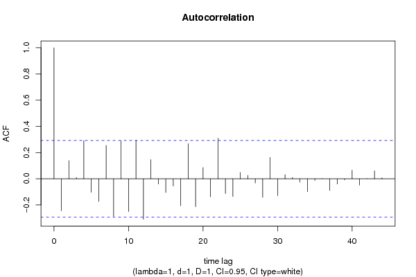
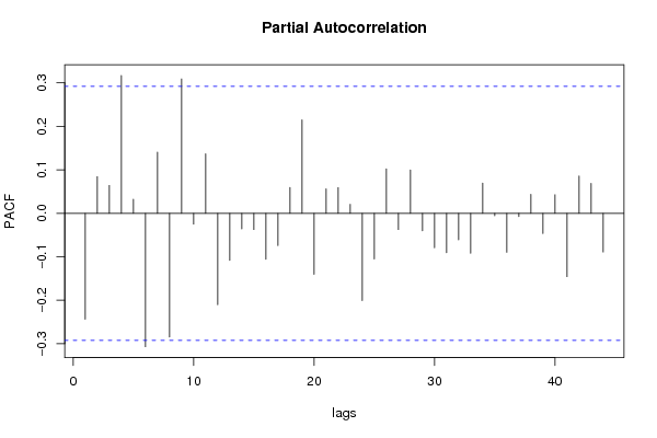
Title produced by software

(Partial) Autocorrelation Function

Date of computation

Fri, 03 Dec 2010 09:44:21 +0000

Cite this page as follows

Statistical Computations at FreeStatistics.org, Office for Research Development and Education, URL https://freestatistics.org/blog/index.php?v=date/2010/Dec/03/t1291369386psiud07fey71utl.htm/, Retrieved Tue, 07 May 2024 21:51:20 +0000

Statistical Computations at FreeStatistics.org, Office for Research Development and Education, URL https://freestatistics.org/blog/index.php?pk=104569, Retrieved Tue, 07 May 2024 21:51:20 +0000

QR Codes:

Paste this QR Code to cite your computation.

Original text written by user:

IsPrivate?

No (this computation is public)

User-defined keywords

Estimated Impact

207

Family? (F = Feedback message, R = changed R code, M = changed R Module, P = changed Parameters, D = changed Data)

-     [Univariate Data Series] [data set] [2008-12-01 19:54:57] [b98453cac15ba1066b407e146608df68]
- RMP   [(Partial) Autocorrelation Function] [Unemployment] [2010-11-29 09:09:37] [b98453cac15ba1066b407e146608df68]
F   PD      [(Partial) Autocorrelation Function] [Autocorrelation F...] [2010-12-03 09:44:21] [e665313c9926a9f4bdf6ad1ee5aefad6] [Current]
-   PD        [(Partial) Autocorrelation Function] [autocorrelatie fu...] [2010-12-18 19:29:00] [74deae64b71f9d77c839af86f7c687b5] 
-   PD        [(Partial) Autocorrelation Function] [autocorrelatie fu...] [2010-12-18 19:36:44] [74deae64b71f9d77c839af86f7c687b5] 
-               [(Partial) Autocorrelation Function] [autocorrelatiefun...] [2010-12-18 20:27:56] [74deae64b71f9d77c839af86f7c687b5] 
- RM          [(Partial) Autocorrelation Function] [] [2011-12-06 18:36:28] [74be16979710d4c4e7c6647856088456] 
- R  D        [(Partial) Autocorrelation Function] [] [2011-12-06 18:37:12] [46d7ccc24e5d35a2decd922dfb3b3a39] 
-               [(Partial) Autocorrelation Function] [] [2011-12-06 18:49:25] [46d7ccc24e5d35a2decd922dfb3b3a39] 

Feedback Forum

2010-12-13 11:24:03 [Stefanie Van Esbroeck] [reply] 
Je maakte een correcte berekening. je paste alle parameters correct aan. Je nam de time lags groot genoeg om de output gemakkelijk te kunnen aflezen en je nam de gevonden waarden uit de vorige berekening over zodat het resultaat verder bouwd op de vorige berekening. goed uitgewerkt. Je interpretatie is correct maar je had deze wel nog kunenn uitbreiden met extra informatie over de grafieken. We zien inderdaad dat er geen autocorrelatie aanwezig is maar je had hier ook de waarden van lags 12,24,36 en 48 kunnen bespreken. Om zo je interpretatie wat meer te onderbouwen. We zien inderdaad dat de trend uit de reeks is gehaald en je zegt ook hoe dit komt maar je zegt wel niet wat uit de grafiek dit aantoont. Je had hier dus ook kunnen aan toevoegen dat er in de eerste 10 lags er geen dalende trend meer zichtbaar is.

Post a new message

Dataseries X:

Download CSV

Histogram

Boxplots

Summary of computational transaction
Raw Input	view raw input (R code)
Raw Output	view raw output of R engine
Computing time	2 seconds
R Server	'Sir Ronald Aylmer Fisher' @ 193.190.124.24

\begin{tabular}{lllllllll}
\hline
Summary of computational transaction \tabularnewline
Raw Input & view raw input (R code)  \tabularnewline
Raw Output & view raw output of R engine  \tabularnewline
Computing time & 2 seconds \tabularnewline
R Server & 'Sir Ronald Aylmer Fisher' @ 193.190.124.24 \tabularnewline
\hline
\end{tabular}
%Source: https://freestatistics.org/blog/index.php?pk=104569&T=0

[TABLE]
[ROW][C]Summary of computational transaction[/C][/ROW]
[ROW][C]Raw Input[/C][C]view raw input (R code) [/C][/ROW]
[ROW][C]Raw Output[/C][C]view raw output of R engine [/C][/ROW]
[ROW][C]Computing time[/C][C]2 seconds[/C][/ROW]
[ROW][C]R Server[/C][C]'Sir Ronald Aylmer Fisher' @ 193.190.124.24[/C][/ROW]
[/TABLE]
Source: https://freestatistics.org/blog/index.php?pk=104569&T=0

Globally Unique Identifier (entire table): ba.freestatistics.org/blog/index.php?pk=104569&T=0

As an alternative you can also use a QR Code:

The GUIDs for individual cells are displayed in the table below:

Summary of computational transaction
Raw Input	view raw input (R code)
Raw Output	view raw output of R engine
Computing time	2 seconds
R Server	'Sir Ronald Aylmer Fisher' @ 193.190.124.24

Autocorrelation Function
Time lag k	ACF(k)	T-STAT	P-value
1	-0.243728	-1.635	0.054515
2	0.138719	0.9306	0.178524
3	0.00837	0.0561	0.477735
4	0.291049	1.9524	0.028563
5	-0.103181	-0.6922	0.246197
6	-0.173061	-1.1609	0.125897
7	0.255001	1.7106	0.047021
8	-0.285695	-1.9165	0.030833
9	0.289763	1.9438	0.029095
10	-0.250304	-1.6791	0.050033
11	0.292178	1.96	0.028103
12	-0.309274	-2.0747	0.021882
13	0.146461	0.9825	0.165556
14	-0.040484	-0.2716	0.393594
15	-0.104534	-0.7012	0.243384
16	-0.055723	-0.3738	0.355153
17	-0.205059	-1.3756	0.08788
18	0.268067	1.7982	0.039424
19	-0.212837	-1.4278	0.080133
20	0.085639	0.5745	0.28425
21	-0.137971	-0.9255	0.179812
22	0.309417	2.0756	0.021836
23	-0.112567	-0.7551	0.227055
24	-0.135622	-0.9098	0.183893
25	0.048221	0.3235	0.373916
26	0.026025	0.1746	0.431095
27	-0.032728	-0.2195	0.413609
28	-0.141388	-0.9485	0.173981
29	0.163741	1.0984	0.138935
30	-0.129348	-0.8677	0.195083
31	0.031714	0.2127	0.416243
32	0.009494	0.0637	0.47475
33	-0.025533	-0.1713	0.432385
34	-0.09876	-0.6625	0.255514
35	-0.012853	-0.0862	0.465836
36	-0.000706	-0.0047	0.498122
37	-0.08916	-0.5981	0.276384
38	-0.039962	-0.2681	0.394934
39	-0.008345	-0.056	0.477801
40	0.065273	0.4379	0.331789
41	-0.048213	-0.3234	0.373936
42	0.000634	0.0043	0.498312
43	0.060518	0.406	0.343345
44	0.006749	0.0453	0.482044
45	NA	NA	NA
46	NA	NA	NA
47	NA	NA	NA
48	NA	NA	NA

\begin{tabular}{lllllllll}
\hline
Autocorrelation Function \tabularnewline
Time lag k & ACF(k) & T-STAT & P-value \tabularnewline
1 & -0.243728 & -1.635 & 0.054515 \tabularnewline
2 & 0.138719 & 0.9306 & 0.178524 \tabularnewline
3 & 0.00837 & 0.0561 & 0.477735 \tabularnewline
4 & 0.291049 & 1.9524 & 0.028563 \tabularnewline
5 & -0.103181 & -0.6922 & 0.246197 \tabularnewline
6 & -0.173061 & -1.1609 & 0.125897 \tabularnewline
7 & 0.255001 & 1.7106 & 0.047021 \tabularnewline
8 & -0.285695 & -1.9165 & 0.030833 \tabularnewline
9 & 0.289763 & 1.9438 & 0.029095 \tabularnewline
10 & -0.250304 & -1.6791 & 0.050033 \tabularnewline
11 & 0.292178 & 1.96 & 0.028103 \tabularnewline
12 & -0.309274 & -2.0747 & 0.021882 \tabularnewline
13 & 0.146461 & 0.9825 & 0.165556 \tabularnewline
14 & -0.040484 & -0.2716 & 0.393594 \tabularnewline
15 & -0.104534 & -0.7012 & 0.243384 \tabularnewline
16 & -0.055723 & -0.3738 & 0.355153 \tabularnewline
17 & -0.205059 & -1.3756 & 0.08788 \tabularnewline
18 & 0.268067 & 1.7982 & 0.039424 \tabularnewline
19 & -0.212837 & -1.4278 & 0.080133 \tabularnewline
20 & 0.085639 & 0.5745 & 0.28425 \tabularnewline
21 & -0.137971 & -0.9255 & 0.179812 \tabularnewline
22 & 0.309417 & 2.0756 & 0.021836 \tabularnewline
23 & -0.112567 & -0.7551 & 0.227055 \tabularnewline
24 & -0.135622 & -0.9098 & 0.183893 \tabularnewline
25 & 0.048221 & 0.3235 & 0.373916 \tabularnewline
26 & 0.026025 & 0.1746 & 0.431095 \tabularnewline
27 & -0.032728 & -0.2195 & 0.413609 \tabularnewline
28 & -0.141388 & -0.9485 & 0.173981 \tabularnewline
29 & 0.163741 & 1.0984 & 0.138935 \tabularnewline
30 & -0.129348 & -0.8677 & 0.195083 \tabularnewline
31 & 0.031714 & 0.2127 & 0.416243 \tabularnewline
32 & 0.009494 & 0.0637 & 0.47475 \tabularnewline
33 & -0.025533 & -0.1713 & 0.432385 \tabularnewline
34 & -0.09876 & -0.6625 & 0.255514 \tabularnewline
35 & -0.012853 & -0.0862 & 0.465836 \tabularnewline
36 & -0.000706 & -0.0047 & 0.498122 \tabularnewline
37 & -0.08916 & -0.5981 & 0.276384 \tabularnewline
38 & -0.039962 & -0.2681 & 0.394934 \tabularnewline
39 & -0.008345 & -0.056 & 0.477801 \tabularnewline
40 & 0.065273 & 0.4379 & 0.331789 \tabularnewline
41 & -0.048213 & -0.3234 & 0.373936 \tabularnewline
42 & 0.000634 & 0.0043 & 0.498312 \tabularnewline
43 & 0.060518 & 0.406 & 0.343345 \tabularnewline
44 & 0.006749 & 0.0453 & 0.482044 \tabularnewline
45 & NA & NA & NA \tabularnewline
46 & NA & NA & NA \tabularnewline
47 & NA & NA & NA \tabularnewline
48 & NA & NA & NA \tabularnewline
\hline
\end{tabular}
%Source: https://freestatistics.org/blog/index.php?pk=104569&T=1

[TABLE]
[ROW][C]Autocorrelation Function[/C][/ROW]
[ROW][C]Time lag k[/C][C]ACF(k)[/C][C]T-STAT[/C][C]P-value[/C][/ROW]
[ROW][C]1[/C][C]-0.243728[/C][C]-1.635[/C][C]0.054515[/C][/ROW]
[ROW][C]2[/C][C]0.138719[/C][C]0.9306[/C][C]0.178524[/C][/ROW]
[ROW][C]3[/C][C]0.00837[/C][C]0.0561[/C][C]0.477735[/C][/ROW]
[ROW][C]4[/C][C]0.291049[/C][C]1.9524[/C][C]0.028563[/C][/ROW]
[ROW][C]5[/C][C]-0.103181[/C][C]-0.6922[/C][C]0.246197[/C][/ROW]
[ROW][C]6[/C][C]-0.173061[/C][C]-1.1609[/C][C]0.125897[/C][/ROW]
[ROW][C]7[/C][C]0.255001[/C][C]1.7106[/C][C]0.047021[/C][/ROW]
[ROW][C]8[/C][C]-0.285695[/C][C]-1.9165[/C][C]0.030833[/C][/ROW]
[ROW][C]9[/C][C]0.289763[/C][C]1.9438[/C][C]0.029095[/C][/ROW]
[ROW][C]10[/C][C]-0.250304[/C][C]-1.6791[/C][C]0.050033[/C][/ROW]
[ROW][C]11[/C][C]0.292178[/C][C]1.96[/C][C]0.028103[/C][/ROW]
[ROW][C]12[/C][C]-0.309274[/C][C]-2.0747[/C][C]0.021882[/C][/ROW]
[ROW][C]13[/C][C]0.146461[/C][C]0.9825[/C][C]0.165556[/C][/ROW]
[ROW][C]14[/C][C]-0.040484[/C][C]-0.2716[/C][C]0.393594[/C][/ROW]
[ROW][C]15[/C][C]-0.104534[/C][C]-0.7012[/C][C]0.243384[/C][/ROW]
[ROW][C]16[/C][C]-0.055723[/C][C]-0.3738[/C][C]0.355153[/C][/ROW]
[ROW][C]17[/C][C]-0.205059[/C][C]-1.3756[/C][C]0.08788[/C][/ROW]
[ROW][C]18[/C][C]0.268067[/C][C]1.7982[/C][C]0.039424[/C][/ROW]
[ROW][C]19[/C][C]-0.212837[/C][C]-1.4278[/C][C]0.080133[/C][/ROW]
[ROW][C]20[/C][C]0.085639[/C][C]0.5745[/C][C]0.28425[/C][/ROW]
[ROW][C]21[/C][C]-0.137971[/C][C]-0.9255[/C][C]0.179812[/C][/ROW]
[ROW][C]22[/C][C]0.309417[/C][C]2.0756[/C][C]0.021836[/C][/ROW]
[ROW][C]23[/C][C]-0.112567[/C][C]-0.7551[/C][C]0.227055[/C][/ROW]
[ROW][C]24[/C][C]-0.135622[/C][C]-0.9098[/C][C]0.183893[/C][/ROW]
[ROW][C]25[/C][C]0.048221[/C][C]0.3235[/C][C]0.373916[/C][/ROW]
[ROW][C]26[/C][C]0.026025[/C][C]0.1746[/C][C]0.431095[/C][/ROW]
[ROW][C]27[/C][C]-0.032728[/C][C]-0.2195[/C][C]0.413609[/C][/ROW]
[ROW][C]28[/C][C]-0.141388[/C][C]-0.9485[/C][C]0.173981[/C][/ROW]
[ROW][C]29[/C][C]0.163741[/C][C]1.0984[/C][C]0.138935[/C][/ROW]
[ROW][C]30[/C][C]-0.129348[/C][C]-0.8677[/C][C]0.195083[/C][/ROW]
[ROW][C]31[/C][C]0.031714[/C][C]0.2127[/C][C]0.416243[/C][/ROW]
[ROW][C]32[/C][C]0.009494[/C][C]0.0637[/C][C]0.47475[/C][/ROW]
[ROW][C]33[/C][C]-0.025533[/C][C]-0.1713[/C][C]0.432385[/C][/ROW]
[ROW][C]34[/C][C]-0.09876[/C][C]-0.6625[/C][C]0.255514[/C][/ROW]
[ROW][C]35[/C][C]-0.012853[/C][C]-0.0862[/C][C]0.465836[/C][/ROW]
[ROW][C]36[/C][C]-0.000706[/C][C]-0.0047[/C][C]0.498122[/C][/ROW]
[ROW][C]37[/C][C]-0.08916[/C][C]-0.5981[/C][C]0.276384[/C][/ROW]
[ROW][C]38[/C][C]-0.039962[/C][C]-0.2681[/C][C]0.394934[/C][/ROW]
[ROW][C]39[/C][C]-0.008345[/C][C]-0.056[/C][C]0.477801[/C][/ROW]
[ROW][C]40[/C][C]0.065273[/C][C]0.4379[/C][C]0.331789[/C][/ROW]
[ROW][C]41[/C][C]-0.048213[/C][C]-0.3234[/C][C]0.373936[/C][/ROW]
[ROW][C]42[/C][C]0.000634[/C][C]0.0043[/C][C]0.498312[/C][/ROW]
[ROW][C]43[/C][C]0.060518[/C][C]0.406[/C][C]0.343345[/C][/ROW]
[ROW][C]44[/C][C]0.006749[/C][C]0.0453[/C][C]0.482044[/C][/ROW]
[ROW][C]45[/C][C]NA[/C][C]NA[/C][C]NA[/C][/ROW]
[ROW][C]46[/C][C]NA[/C][C]NA[/C][C]NA[/C][/ROW]
[ROW][C]47[/C][C]NA[/C][C]NA[/C][C]NA[/C][/ROW]
[ROW][C]48[/C][C]NA[/C][C]NA[/C][C]NA[/C][/ROW]
[/TABLE]
Source: https://freestatistics.org/blog/index.php?pk=104569&T=1

Globally Unique Identifier (entire table): ba.freestatistics.org/blog/index.php?pk=104569&T=1

As an alternative you can also use a QR Code:

The GUIDs for individual cells are displayed in the table below:

Autocorrelation Function
Time lag k	ACF(k)	T-STAT	P-value
1	-0.243728	-1.635	0.054515
2	0.138719	0.9306	0.178524
3	0.00837	0.0561	0.477735
4	0.291049	1.9524	0.028563
5	-0.103181	-0.6922	0.246197
6	-0.173061	-1.1609	0.125897
7	0.255001	1.7106	0.047021
8	-0.285695	-1.9165	0.030833
9	0.289763	1.9438	0.029095
10	-0.250304	-1.6791	0.050033
11	0.292178	1.96	0.028103
12	-0.309274	-2.0747	0.021882
13	0.146461	0.9825	0.165556
14	-0.040484	-0.2716	0.393594
15	-0.104534	-0.7012	0.243384
16	-0.055723	-0.3738	0.355153
17	-0.205059	-1.3756	0.08788
18	0.268067	1.7982	0.039424
19	-0.212837	-1.4278	0.080133
20	0.085639	0.5745	0.28425
21	-0.137971	-0.9255	0.179812
22	0.309417	2.0756	0.021836
23	-0.112567	-0.7551	0.227055
24	-0.135622	-0.9098	0.183893
25	0.048221	0.3235	0.373916
26	0.026025	0.1746	0.431095
27	-0.032728	-0.2195	0.413609
28	-0.141388	-0.9485	0.173981
29	0.163741	1.0984	0.138935
30	-0.129348	-0.8677	0.195083
31	0.031714	0.2127	0.416243
32	0.009494	0.0637	0.47475
33	-0.025533	-0.1713	0.432385
34	-0.09876	-0.6625	0.255514
35	-0.012853	-0.0862	0.465836
36	-0.000706	-0.0047	0.498122
37	-0.08916	-0.5981	0.276384
38	-0.039962	-0.2681	0.394934
39	-0.008345	-0.056	0.477801
40	0.065273	0.4379	0.331789
41	-0.048213	-0.3234	0.373936
42	0.000634	0.0043	0.498312
43	0.060518	0.406	0.343345
44	0.006749	0.0453	0.482044
45	NA	NA	NA
46	NA	NA	NA
47	NA	NA	NA
48	NA	NA	NA

Partial Autocorrelation Function
Time lag k	PACF(k)	T-STAT	P-value
1	-0.243728	-1.635	0.054515
2	0.084325	0.5657	0.287213
3	0.064119	0.4301	0.334579
4	0.317081	2.127	0.019466
5	0.032316	0.2168	0.41468
6	-0.306899	-2.0587	0.022668
7	0.140553	0.9429	0.175395
8	-0.284631	-1.9094	0.031302
9	0.309142	2.0738	0.021926
10	-0.02482	-0.1665	0.434257
11	0.136938	0.9186	0.1816
12	-0.210219	-1.4102	0.082679
13	-0.108258	-0.7262	0.235733
14	-0.035796	-0.2401	0.405661
15	-0.037297	-0.2502	0.401787
16	-0.105714	-0.7092	0.240945
17	-0.074201	-0.4978	0.31054
18	0.059247	0.3974	0.346461
19	0.214967	1.442	0.078108
20	-0.140106	-0.9399	0.176153
21	0.056535	0.3792	0.353144
22	0.059177	0.397	0.346631
23	0.020793	0.1395	0.444846
24	-0.200883	-1.3476	0.092272
25	-0.105042	-0.7046	0.242332
26	0.102399	0.6869	0.247831
27	-0.037339	-0.2505	0.401679
28	0.099539	0.6677	0.25386
29	-0.04036	-0.2707	0.393913
30	-0.079138	-0.5309	0.299059
31	-0.090501	-0.6071	0.273418
32	-0.060934	-0.4088	0.342328
33	-0.09203	-0.6174	0.270055
34	0.069359	0.4653	0.321989
35	-0.005407	-0.0363	0.485615
36	-0.089661	-0.6015	0.275275
37	-0.007434	-0.0499	0.480225
38	0.043665	0.2929	0.385468
39	-0.046695	-0.3132	0.377774
40	0.042832	0.2873	0.38759
41	-0.145712	-0.9775	0.166781
42	0.086017	0.577	0.283402
43	0.068961	0.4626	0.322938
44	-0.088976	-0.5969	0.276793
45	NA	NA	NA
46	NA	NA	NA
47	NA	NA	NA
48	NA	NA	NA

\begin{tabular}{lllllllll}
\hline
Partial Autocorrelation Function \tabularnewline
Time lag k & PACF(k) & T-STAT & P-value \tabularnewline
1 & -0.243728 & -1.635 & 0.054515 \tabularnewline
2 & 0.084325 & 0.5657 & 0.287213 \tabularnewline
3 & 0.064119 & 0.4301 & 0.334579 \tabularnewline
4 & 0.317081 & 2.127 & 0.019466 \tabularnewline
5 & 0.032316 & 0.2168 & 0.41468 \tabularnewline
6 & -0.306899 & -2.0587 & 0.022668 \tabularnewline
7 & 0.140553 & 0.9429 & 0.175395 \tabularnewline
8 & -0.284631 & -1.9094 & 0.031302 \tabularnewline
9 & 0.309142 & 2.0738 & 0.021926 \tabularnewline
10 & -0.02482 & -0.1665 & 0.434257 \tabularnewline
11 & 0.136938 & 0.9186 & 0.1816 \tabularnewline
12 & -0.210219 & -1.4102 & 0.082679 \tabularnewline
13 & -0.108258 & -0.7262 & 0.235733 \tabularnewline
14 & -0.035796 & -0.2401 & 0.405661 \tabularnewline
15 & -0.037297 & -0.2502 & 0.401787 \tabularnewline
16 & -0.105714 & -0.7092 & 0.240945 \tabularnewline
17 & -0.074201 & -0.4978 & 0.31054 \tabularnewline
18 & 0.059247 & 0.3974 & 0.346461 \tabularnewline
19 & 0.214967 & 1.442 & 0.078108 \tabularnewline
20 & -0.140106 & -0.9399 & 0.176153 \tabularnewline
21 & 0.056535 & 0.3792 & 0.353144 \tabularnewline
22 & 0.059177 & 0.397 & 0.346631 \tabularnewline
23 & 0.020793 & 0.1395 & 0.444846 \tabularnewline
24 & -0.200883 & -1.3476 & 0.092272 \tabularnewline
25 & -0.105042 & -0.7046 & 0.242332 \tabularnewline
26 & 0.102399 & 0.6869 & 0.247831 \tabularnewline
27 & -0.037339 & -0.2505 & 0.401679 \tabularnewline
28 & 0.099539 & 0.6677 & 0.25386 \tabularnewline
29 & -0.04036 & -0.2707 & 0.393913 \tabularnewline
30 & -0.079138 & -0.5309 & 0.299059 \tabularnewline
31 & -0.090501 & -0.6071 & 0.273418 \tabularnewline
32 & -0.060934 & -0.4088 & 0.342328 \tabularnewline
33 & -0.09203 & -0.6174 & 0.270055 \tabularnewline
34 & 0.069359 & 0.4653 & 0.321989 \tabularnewline
35 & -0.005407 & -0.0363 & 0.485615 \tabularnewline
36 & -0.089661 & -0.6015 & 0.275275 \tabularnewline
37 & -0.007434 & -0.0499 & 0.480225 \tabularnewline
38 & 0.043665 & 0.2929 & 0.385468 \tabularnewline
39 & -0.046695 & -0.3132 & 0.377774 \tabularnewline
40 & 0.042832 & 0.2873 & 0.38759 \tabularnewline
41 & -0.145712 & -0.9775 & 0.166781 \tabularnewline
42 & 0.086017 & 0.577 & 0.283402 \tabularnewline
43 & 0.068961 & 0.4626 & 0.322938 \tabularnewline
44 & -0.088976 & -0.5969 & 0.276793 \tabularnewline
45 & NA & NA & NA \tabularnewline
46 & NA & NA & NA \tabularnewline
47 & NA & NA & NA \tabularnewline
48 & NA & NA & NA \tabularnewline
\hline
\end{tabular}
%Source: https://freestatistics.org/blog/index.php?pk=104569&T=2

[TABLE]
[ROW][C]Partial Autocorrelation Function[/C][/ROW]
[ROW][C]Time lag k[/C][C]PACF(k)[/C][C]T-STAT[/C][C]P-value[/C][/ROW]
[ROW][C]1[/C][C]-0.243728[/C][C]-1.635[/C][C]0.054515[/C][/ROW]
[ROW][C]2[/C][C]0.084325[/C][C]0.5657[/C][C]0.287213[/C][/ROW]
[ROW][C]3[/C][C]0.064119[/C][C]0.4301[/C][C]0.334579[/C][/ROW]
[ROW][C]4[/C][C]0.317081[/C][C]2.127[/C][C]0.019466[/C][/ROW]
[ROW][C]5[/C][C]0.032316[/C][C]0.2168[/C][C]0.41468[/C][/ROW]
[ROW][C]6[/C][C]-0.306899[/C][C]-2.0587[/C][C]0.022668[/C][/ROW]
[ROW][C]7[/C][C]0.140553[/C][C]0.9429[/C][C]0.175395[/C][/ROW]
[ROW][C]8[/C][C]-0.284631[/C][C]-1.9094[/C][C]0.031302[/C][/ROW]
[ROW][C]9[/C][C]0.309142[/C][C]2.0738[/C][C]0.021926[/C][/ROW]
[ROW][C]10[/C][C]-0.02482[/C][C]-0.1665[/C][C]0.434257[/C][/ROW]
[ROW][C]11[/C][C]0.136938[/C][C]0.9186[/C][C]0.1816[/C][/ROW]
[ROW][C]12[/C][C]-0.210219[/C][C]-1.4102[/C][C]0.082679[/C][/ROW]
[ROW][C]13[/C][C]-0.108258[/C][C]-0.7262[/C][C]0.235733[/C][/ROW]
[ROW][C]14[/C][C]-0.035796[/C][C]-0.2401[/C][C]0.405661[/C][/ROW]
[ROW][C]15[/C][C]-0.037297[/C][C]-0.2502[/C][C]0.401787[/C][/ROW]
[ROW][C]16[/C][C]-0.105714[/C][C]-0.7092[/C][C]0.240945[/C][/ROW]
[ROW][C]17[/C][C]-0.074201[/C][C]-0.4978[/C][C]0.31054[/C][/ROW]
[ROW][C]18[/C][C]0.059247[/C][C]0.3974[/C][C]0.346461[/C][/ROW]
[ROW][C]19[/C][C]0.214967[/C][C]1.442[/C][C]0.078108[/C][/ROW]
[ROW][C]20[/C][C]-0.140106[/C][C]-0.9399[/C][C]0.176153[/C][/ROW]
[ROW][C]21[/C][C]0.056535[/C][C]0.3792[/C][C]0.353144[/C][/ROW]
[ROW][C]22[/C][C]0.059177[/C][C]0.397[/C][C]0.346631[/C][/ROW]
[ROW][C]23[/C][C]0.020793[/C][C]0.1395[/C][C]0.444846[/C][/ROW]
[ROW][C]24[/C][C]-0.200883[/C][C]-1.3476[/C][C]0.092272[/C][/ROW]
[ROW][C]25[/C][C]-0.105042[/C][C]-0.7046[/C][C]0.242332[/C][/ROW]
[ROW][C]26[/C][C]0.102399[/C][C]0.6869[/C][C]0.247831[/C][/ROW]
[ROW][C]27[/C][C]-0.037339[/C][C]-0.2505[/C][C]0.401679[/C][/ROW]
[ROW][C]28[/C][C]0.099539[/C][C]0.6677[/C][C]0.25386[/C][/ROW]
[ROW][C]29[/C][C]-0.04036[/C][C]-0.2707[/C][C]0.393913[/C][/ROW]
[ROW][C]30[/C][C]-0.079138[/C][C]-0.5309[/C][C]0.299059[/C][/ROW]
[ROW][C]31[/C][C]-0.090501[/C][C]-0.6071[/C][C]0.273418[/C][/ROW]
[ROW][C]32[/C][C]-0.060934[/C][C]-0.4088[/C][C]0.342328[/C][/ROW]
[ROW][C]33[/C][C]-0.09203[/C][C]-0.6174[/C][C]0.270055[/C][/ROW]
[ROW][C]34[/C][C]0.069359[/C][C]0.4653[/C][C]0.321989[/C][/ROW]
[ROW][C]35[/C][C]-0.005407[/C][C]-0.0363[/C][C]0.485615[/C][/ROW]
[ROW][C]36[/C][C]-0.089661[/C][C]-0.6015[/C][C]0.275275[/C][/ROW]
[ROW][C]37[/C][C]-0.007434[/C][C]-0.0499[/C][C]0.480225[/C][/ROW]
[ROW][C]38[/C][C]0.043665[/C][C]0.2929[/C][C]0.385468[/C][/ROW]
[ROW][C]39[/C][C]-0.046695[/C][C]-0.3132[/C][C]0.377774[/C][/ROW]
[ROW][C]40[/C][C]0.042832[/C][C]0.2873[/C][C]0.38759[/C][/ROW]
[ROW][C]41[/C][C]-0.145712[/C][C]-0.9775[/C][C]0.166781[/C][/ROW]
[ROW][C]42[/C][C]0.086017[/C][C]0.577[/C][C]0.283402[/C][/ROW]
[ROW][C]43[/C][C]0.068961[/C][C]0.4626[/C][C]0.322938[/C][/ROW]
[ROW][C]44[/C][C]-0.088976[/C][C]-0.5969[/C][C]0.276793[/C][/ROW]
[ROW][C]45[/C][C]NA[/C][C]NA[/C][C]NA[/C][/ROW]
[ROW][C]46[/C][C]NA[/C][C]NA[/C][C]NA[/C][/ROW]
[ROW][C]47[/C][C]NA[/C][C]NA[/C][C]NA[/C][/ROW]
[ROW][C]48[/C][C]NA[/C][C]NA[/C][C]NA[/C][/ROW]
[/TABLE]
Source: https://freestatistics.org/blog/index.php?pk=104569&T=2

Globally Unique Identifier (entire table): ba.freestatistics.org/blog/index.php?pk=104569&T=2

As an alternative you can also use a QR Code:

The GUIDs for individual cells are displayed in the table below:

Partial Autocorrelation Function
Time lag k	PACF(k)	T-STAT	P-value
1	-0.243728	-1.635	0.054515
2	0.084325	0.5657	0.287213
3	0.064119	0.4301	0.334579
4	0.317081	2.127	0.019466
5	0.032316	0.2168	0.41468
6	-0.306899	-2.0587	0.022668
7	0.140553	0.9429	0.175395
8	-0.284631	-1.9094	0.031302
9	0.309142	2.0738	0.021926
10	-0.02482	-0.1665	0.434257
11	0.136938	0.9186	0.1816
12	-0.210219	-1.4102	0.082679
13	-0.108258	-0.7262	0.235733
14	-0.035796	-0.2401	0.405661
15	-0.037297	-0.2502	0.401787
16	-0.105714	-0.7092	0.240945
17	-0.074201	-0.4978	0.31054
18	0.059247	0.3974	0.346461
19	0.214967	1.442	0.078108
20	-0.140106	-0.9399	0.176153
21	0.056535	0.3792	0.353144
22	0.059177	0.397	0.346631
23	0.020793	0.1395	0.444846
24	-0.200883	-1.3476	0.092272
25	-0.105042	-0.7046	0.242332
26	0.102399	0.6869	0.247831
27	-0.037339	-0.2505	0.401679
28	0.099539	0.6677	0.25386
29	-0.04036	-0.2707	0.393913
30	-0.079138	-0.5309	0.299059
31	-0.090501	-0.6071	0.273418
32	-0.060934	-0.4088	0.342328
33	-0.09203	-0.6174	0.270055
34	0.069359	0.4653	0.321989
35	-0.005407	-0.0363	0.485615
36	-0.089661	-0.6015	0.275275
37	-0.007434	-0.0499	0.480225
38	0.043665	0.2929	0.385468
39	-0.046695	-0.3132	0.377774
40	0.042832	0.2873	0.38759
41	-0.145712	-0.9775	0.166781
42	0.086017	0.577	0.283402
43	0.068961	0.4626	0.322938
44	-0.088976	-0.5969	0.276793
45	NA	NA	NA
46	NA	NA	NA
47	NA	NA	NA
48	NA	NA	NA

Figure 1

PNG link

Postscript link

PDF link

Figure 2

PNG link

Postscript link

PDF link

Parameters (Session):

par1 = 48 ; par2 = 1 ; par3 = 1 ; par4 = 1 ; par5 = 12 ; par6 = White Noise ; par7 = 0.95 ;

Parameters (R input):

par1 = 48 ; par2 = 1 ; par3 = 1 ; par4 = 1 ; par5 = 12 ; par6 = White Noise ; par7 = 0.95 ;

R code (references can be found in the software module):

if (par1 == 'Default') {
par1 = 10*log10(length(x))
} else {
par1 <- as.numeric(par1)
}
par2 <- as.numeric(par2)
par3 <- as.numeric(par3)
par4 <- as.numeric(par4)
par5 <- as.numeric(par5)
if (par6 == 'White Noise') par6 <- 'white' else par6 <- 'ma'
par7 <- as.numeric(par7)
if (par2 == 0) {
x <- log(x)
} else {
x <- (x ^ par2 - 1) / par2
}
if (par3 > 0) x <- diff(x,lag=1,difference=par3)
if (par4 > 0) x <- diff(x,lag=par5,difference=par4)
bitmap(file='pic1.png')
racf <- acf(x, par1, main='Autocorrelation', xlab='time lag', ylab='ACF', ci.type=par6, ci=par7, sub=paste('(lambda=',par2,', d=',par3,', D=',par4,', CI=', par7, ', CI type=',par6,')',sep=''))
dev.off()
bitmap(file='pic2.png')
rpacf <- pacf(x,par1,main='Partial Autocorrelation',xlab='lags',ylab='PACF')
dev.off()
(myacf <- c(racf$acf))
(mypacf <- c(rpacf$acf))
lengthx <- length(x)
sqrtn <- sqrt(lengthx)
load(file='createtable')
a<-table.start()
a<-table.row.start(a)
a<-table.element(a,'Autocorrelation Function',4,TRUE)
a<-table.row.end(a)
a<-table.row.start(a)
a<-table.element(a,'Time lag k',header=TRUE)
a<-table.element(a,hyperlink('basics.htm','ACF(k)','click here for more information about the Autocorrelation Function'),header=TRUE)
a<-table.element(a,'T-STAT',header=TRUE)
a<-table.element(a,'P-value',header=TRUE)
a<-table.row.end(a)
for (i in 2:(par1+1)) {
a<-table.row.start(a)
a<-table.element(a,i-1,header=TRUE)
a<-table.element(a,round(myacf[i],6))
mytstat <- myacf[i]*sqrtn
a<-table.element(a,round(mytstat,4))
a<-table.element(a,round(1-pt(abs(mytstat),lengthx),6))
a<-table.row.end(a)
}
a<-table.end(a)
table.save(a,file='mytable.tab')
a<-table.start()
a<-table.row.start(a)
a<-table.element(a,'Partial Autocorrelation Function',4,TRUE)
a<-table.row.end(a)
a<-table.row.start(a)
a<-table.element(a,'Time lag k',header=TRUE)
a<-table.element(a,hyperlink('basics.htm','PACF(k)','click here for more information about the Partial Autocorrelation Function'),header=TRUE)
a<-table.element(a,'T-STAT',header=TRUE)
a<-table.element(a,'P-value',header=TRUE)
a<-table.row.end(a)
for (i in 1:par1) {
a<-table.row.start(a)
a<-table.element(a,i,header=TRUE)
a<-table.element(a,round(mypacf[i],6))
mytstat <- mypacf[i]*sqrtn
a<-table.element(a,round(mytstat,4))
a<-table.element(a,round(1-pt(abs(mytstat),lengthx),6))
a<-table.row.end(a)
}
a<-table.end(a)
table.save(a,file='mytable1.tab')

Free Statistics

Description of Statistical Computation

Tree of Dependent Computations

Dataset

Tables (Output of Computation)

Figures (Output of Computation)

Input Parameters & R Code