Repository of Reproducible Computations

Free Statistics

of Irreproducible Research!

Author's title

Author

*The author of this computation has been verified*

R Software Module

rwasp_autocorrelation.wasp

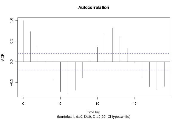
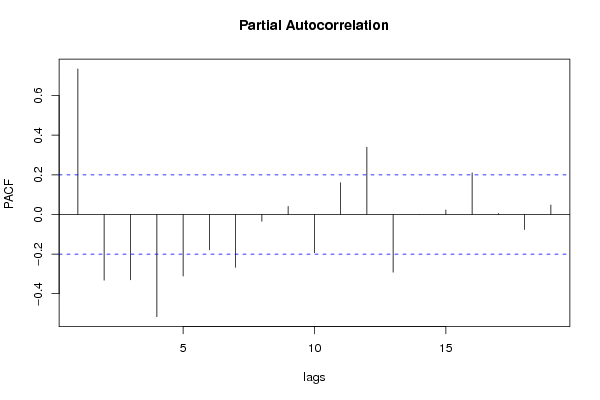
Title produced by software

(Partial) Autocorrelation Function

Date of computation

Fri, 03 Dec 2010 09:35:35 +0000

Cite this page as follows

Statistical Computations at FreeStatistics.org, Office for Research Development and Education, URL https://freestatistics.org/blog/index.php?v=date/2010/Dec/03/t1291368837bjzjgk8laj7m6n2.htm/, Retrieved Tue, 07 May 2024 05:57:08 +0000

Statistical Computations at FreeStatistics.org, Office for Research Development and Education, URL https://freestatistics.org/blog/index.php?pk=104558, Retrieved Tue, 07 May 2024 05:57:08 +0000

QR Codes:

Paste this QR Code to cite your computation.

Original text written by user:

IsPrivate?

No (this computation is public)

User-defined keywords

Estimated Impact

133

Family? (F = Feedback message, R = changed R code, M = changed R Module, P = changed Parameters, D = changed Data)

-     [Univariate Explorative Data Analysis] [Run Sequence gebo...] [2008-12-12 13:32:37] [76963dc1903f0f612b6153510a3818cf]
- R  D  [Univariate Explorative Data Analysis] [Run Sequence gebo...] [2008-12-17 12:14:40] [76963dc1903f0f612b6153510a3818cf]
-         [Univariate Explorative Data Analysis] [Run Sequence Plot...] [2008-12-22 18:19:51] [1ce0d16c8f4225c977b42c8fa93bc163]
- RMP       [Univariate Data Series] [Identifying Integ...] [2009-11-22 12:08:06] [b98453cac15ba1066b407e146608df68]
- RMP         [(Partial) Autocorrelation Function] [Births] [2010-11-29 09:36:27] [b98453cac15ba1066b407e146608df68]
- R PD            [(Partial) Autocorrelation Function] [ACF (Huwelijken)] [2010-12-03 09:35:35] [3de277db83c2673156e9464be2ef6f69] [Current]

Feedback Forum

Post a new message

Dataseries X:

Download CSV

Histogram

Boxplots

Summary of computational transaction
Raw Input	view raw input (R code)
Raw Output	view raw output of R engine
Computing time	1 seconds
R Server	'Gwilym Jenkins' @ 72.249.127.135

\begin{tabular}{lllllllll}
\hline
Summary of computational transaction \tabularnewline
Raw Input & view raw input (R code)  \tabularnewline
Raw Output & view raw output of R engine  \tabularnewline
Computing time & 1 seconds \tabularnewline
R Server & 'Gwilym Jenkins' @ 72.249.127.135 \tabularnewline
\hline
\end{tabular}
%Source: https://freestatistics.org/blog/index.php?pk=104558&T=0

[TABLE]
[ROW][C]Summary of computational transaction[/C][/ROW]
[ROW][C]Raw Input[/C][C]view raw input (R code) [/C][/ROW]
[ROW][C]Raw Output[/C][C]view raw output of R engine [/C][/ROW]
[ROW][C]Computing time[/C][C]1 seconds[/C][/ROW]
[ROW][C]R Server[/C][C]'Gwilym Jenkins' @ 72.249.127.135[/C][/ROW]
[/TABLE]
Source: https://freestatistics.org/blog/index.php?pk=104558&T=0

Globally Unique Identifier (entire table): ba.freestatistics.org/blog/index.php?pk=104558&T=0

As an alternative you can also use a QR Code:

The GUIDs for individual cells are displayed in the table below:

Summary of computational transaction
Raw Input	view raw input (R code)
Raw Output	view raw output of R engine
Computing time	1 seconds
R Server	'Gwilym Jenkins' @ 72.249.127.135

Autocorrelation Function
Time lag k	ACF(k)	T-STAT	P-value
1	0.7347	7.1986	0
2	0.387088	3.7927	0.00013
3	-0.000125	-0.0012	0.499511
4	-0.434319	-4.2554	2.4e-05
5	-0.7201	-7.0555	0
6	-0.785135	-7.6927	0
7	-0.692733	-6.7874	0
8	-0.383629	-3.7588	0.000147
9	0.034958	0.3425	0.366357
10	0.356281	3.4908	0.000365
11	0.652426	6.3924	0
12	0.822157	8.0555	0
13	0.623638	6.1104	0
14	0.334269	3.2752	0.000735
15	-0.013351	-0.1308	0.448097
16	-0.364028	-3.5667	0.000283
17	-0.6031	-5.9091	0
18	-0.677232	-6.6355	0
19	-0.596272	-5.8422	0

\begin{tabular}{lllllllll}
\hline
Autocorrelation Function \tabularnewline
Time lag k & ACF(k) & T-STAT & P-value \tabularnewline
1 & 0.7347 & 7.1986 & 0 \tabularnewline
2 & 0.387088 & 3.7927 & 0.00013 \tabularnewline
3 & -0.000125 & -0.0012 & 0.499511 \tabularnewline
4 & -0.434319 & -4.2554 & 2.4e-05 \tabularnewline
5 & -0.7201 & -7.0555 & 0 \tabularnewline
6 & -0.785135 & -7.6927 & 0 \tabularnewline
7 & -0.692733 & -6.7874 & 0 \tabularnewline
8 & -0.383629 & -3.7588 & 0.000147 \tabularnewline
9 & 0.034958 & 0.3425 & 0.366357 \tabularnewline
10 & 0.356281 & 3.4908 & 0.000365 \tabularnewline
11 & 0.652426 & 6.3924 & 0 \tabularnewline
12 & 0.822157 & 8.0555 & 0 \tabularnewline
13 & 0.623638 & 6.1104 & 0 \tabularnewline
14 & 0.334269 & 3.2752 & 0.000735 \tabularnewline
15 & -0.013351 & -0.1308 & 0.448097 \tabularnewline
16 & -0.364028 & -3.5667 & 0.000283 \tabularnewline
17 & -0.6031 & -5.9091 & 0 \tabularnewline
18 & -0.677232 & -6.6355 & 0 \tabularnewline
19 & -0.596272 & -5.8422 & 0 \tabularnewline
\hline
\end{tabular}
%Source: https://freestatistics.org/blog/index.php?pk=104558&T=1

[TABLE]
[ROW][C]Autocorrelation Function[/C][/ROW]
[ROW][C]Time lag k[/C][C]ACF(k)[/C][C]T-STAT[/C][C]P-value[/C][/ROW]
[ROW][C]1[/C][C]0.7347[/C][C]7.1986[/C][C]0[/C][/ROW]
[ROW][C]2[/C][C]0.387088[/C][C]3.7927[/C][C]0.00013[/C][/ROW]
[ROW][C]3[/C][C]-0.000125[/C][C]-0.0012[/C][C]0.499511[/C][/ROW]
[ROW][C]4[/C][C]-0.434319[/C][C]-4.2554[/C][C]2.4e-05[/C][/ROW]
[ROW][C]5[/C][C]-0.7201[/C][C]-7.0555[/C][C]0[/C][/ROW]
[ROW][C]6[/C][C]-0.785135[/C][C]-7.6927[/C][C]0[/C][/ROW]
[ROW][C]7[/C][C]-0.692733[/C][C]-6.7874[/C][C]0[/C][/ROW]
[ROW][C]8[/C][C]-0.383629[/C][C]-3.7588[/C][C]0.000147[/C][/ROW]
[ROW][C]9[/C][C]0.034958[/C][C]0.3425[/C][C]0.366357[/C][/ROW]
[ROW][C]10[/C][C]0.356281[/C][C]3.4908[/C][C]0.000365[/C][/ROW]
[ROW][C]11[/C][C]0.652426[/C][C]6.3924[/C][C]0[/C][/ROW]
[ROW][C]12[/C][C]0.822157[/C][C]8.0555[/C][C]0[/C][/ROW]
[ROW][C]13[/C][C]0.623638[/C][C]6.1104[/C][C]0[/C][/ROW]
[ROW][C]14[/C][C]0.334269[/C][C]3.2752[/C][C]0.000735[/C][/ROW]
[ROW][C]15[/C][C]-0.013351[/C][C]-0.1308[/C][C]0.448097[/C][/ROW]
[ROW][C]16[/C][C]-0.364028[/C][C]-3.5667[/C][C]0.000283[/C][/ROW]
[ROW][C]17[/C][C]-0.6031[/C][C]-5.9091[/C][C]0[/C][/ROW]
[ROW][C]18[/C][C]-0.677232[/C][C]-6.6355[/C][C]0[/C][/ROW]
[ROW][C]19[/C][C]-0.596272[/C][C]-5.8422[/C][C]0[/C][/ROW]
[/TABLE]
Source: https://freestatistics.org/blog/index.php?pk=104558&T=1

Globally Unique Identifier (entire table): ba.freestatistics.org/blog/index.php?pk=104558&T=1

As an alternative you can also use a QR Code:

The GUIDs for individual cells are displayed in the table below:

Autocorrelation Function
Time lag k	ACF(k)	T-STAT	P-value
1	0.7347	7.1986	0
2	0.387088	3.7927	0.00013
3	-0.000125	-0.0012	0.499511
4	-0.434319	-4.2554	2.4e-05
5	-0.7201	-7.0555	0
6	-0.785135	-7.6927	0
7	-0.692733	-6.7874	0
8	-0.383629	-3.7588	0.000147
9	0.034958	0.3425	0.366357
10	0.356281	3.4908	0.000365
11	0.652426	6.3924	0
12	0.822157	8.0555	0
13	0.623638	6.1104	0
14	0.334269	3.2752	0.000735
15	-0.013351	-0.1308	0.448097
16	-0.364028	-3.5667	0.000283
17	-0.6031	-5.9091	0
18	-0.677232	-6.6355	0
19	-0.596272	-5.8422	0

Partial Autocorrelation Function
Time lag k	PACF(k)	T-STAT	P-value
1	0.7347	7.1986	0
2	-0.331793	-3.2509	0.000794
3	-0.329898	-3.2323	0.000842
4	-0.51606	-5.0563	1e-06
5	-0.311301	-3.0501	0.001478
6	-0.178836	-1.7522	0.041464
7	-0.267022	-2.6163	0.005163
8	-0.034569	-0.3387	0.367784
9	0.040271	0.3946	0.347018
10	-0.193038	-1.8914	0.030794
11	0.160128	1.5689	0.059978
12	0.33961	3.3275	0.000622
13	-0.291879	-2.8598	0.0026
14	0.000284	0.0028	0.498892
15	0.022561	0.2211	0.41276
16	0.210063	2.0582	0.021141
17	0.005367	0.0526	0.479086
18	-0.076259	-0.7472	0.228391
19	0.048258	0.4728	0.318703

\begin{tabular}{lllllllll}
\hline
Partial Autocorrelation Function \tabularnewline
Time lag k & PACF(k) & T-STAT & P-value \tabularnewline
1 & 0.7347 & 7.1986 & 0 \tabularnewline
2 & -0.331793 & -3.2509 & 0.000794 \tabularnewline
3 & -0.329898 & -3.2323 & 0.000842 \tabularnewline
4 & -0.51606 & -5.0563 & 1e-06 \tabularnewline
5 & -0.311301 & -3.0501 & 0.001478 \tabularnewline
6 & -0.178836 & -1.7522 & 0.041464 \tabularnewline
7 & -0.267022 & -2.6163 & 0.005163 \tabularnewline
8 & -0.034569 & -0.3387 & 0.367784 \tabularnewline
9 & 0.040271 & 0.3946 & 0.347018 \tabularnewline
10 & -0.193038 & -1.8914 & 0.030794 \tabularnewline
11 & 0.160128 & 1.5689 & 0.059978 \tabularnewline
12 & 0.33961 & 3.3275 & 0.000622 \tabularnewline
13 & -0.291879 & -2.8598 & 0.0026 \tabularnewline
14 & 0.000284 & 0.0028 & 0.498892 \tabularnewline
15 & 0.022561 & 0.2211 & 0.41276 \tabularnewline
16 & 0.210063 & 2.0582 & 0.021141 \tabularnewline
17 & 0.005367 & 0.0526 & 0.479086 \tabularnewline
18 & -0.076259 & -0.7472 & 0.228391 \tabularnewline
19 & 0.048258 & 0.4728 & 0.318703 \tabularnewline
\hline
\end{tabular}
%Source: https://freestatistics.org/blog/index.php?pk=104558&T=2

[TABLE]
[ROW][C]Partial Autocorrelation Function[/C][/ROW]
[ROW][C]Time lag k[/C][C]PACF(k)[/C][C]T-STAT[/C][C]P-value[/C][/ROW]
[ROW][C]1[/C][C]0.7347[/C][C]7.1986[/C][C]0[/C][/ROW]
[ROW][C]2[/C][C]-0.331793[/C][C]-3.2509[/C][C]0.000794[/C][/ROW]
[ROW][C]3[/C][C]-0.329898[/C][C]-3.2323[/C][C]0.000842[/C][/ROW]
[ROW][C]4[/C][C]-0.51606[/C][C]-5.0563[/C][C]1e-06[/C][/ROW]
[ROW][C]5[/C][C]-0.311301[/C][C]-3.0501[/C][C]0.001478[/C][/ROW]
[ROW][C]6[/C][C]-0.178836[/C][C]-1.7522[/C][C]0.041464[/C][/ROW]
[ROW][C]7[/C][C]-0.267022[/C][C]-2.6163[/C][C]0.005163[/C][/ROW]
[ROW][C]8[/C][C]-0.034569[/C][C]-0.3387[/C][C]0.367784[/C][/ROW]
[ROW][C]9[/C][C]0.040271[/C][C]0.3946[/C][C]0.347018[/C][/ROW]
[ROW][C]10[/C][C]-0.193038[/C][C]-1.8914[/C][C]0.030794[/C][/ROW]
[ROW][C]11[/C][C]0.160128[/C][C]1.5689[/C][C]0.059978[/C][/ROW]
[ROW][C]12[/C][C]0.33961[/C][C]3.3275[/C][C]0.000622[/C][/ROW]
[ROW][C]13[/C][C]-0.291879[/C][C]-2.8598[/C][C]0.0026[/C][/ROW]
[ROW][C]14[/C][C]0.000284[/C][C]0.0028[/C][C]0.498892[/C][/ROW]
[ROW][C]15[/C][C]0.022561[/C][C]0.2211[/C][C]0.41276[/C][/ROW]
[ROW][C]16[/C][C]0.210063[/C][C]2.0582[/C][C]0.021141[/C][/ROW]
[ROW][C]17[/C][C]0.005367[/C][C]0.0526[/C][C]0.479086[/C][/ROW]
[ROW][C]18[/C][C]-0.076259[/C][C]-0.7472[/C][C]0.228391[/C][/ROW]
[ROW][C]19[/C][C]0.048258[/C][C]0.4728[/C][C]0.318703[/C][/ROW]
[/TABLE]
Source: https://freestatistics.org/blog/index.php?pk=104558&T=2

Globally Unique Identifier (entire table): ba.freestatistics.org/blog/index.php?pk=104558&T=2

As an alternative you can also use a QR Code:

The GUIDs for individual cells are displayed in the table below:

Partial Autocorrelation Function
Time lag k	PACF(k)	T-STAT	P-value
1	0.7347	7.1986	0
2	-0.331793	-3.2509	0.000794
3	-0.329898	-3.2323	0.000842
4	-0.51606	-5.0563	1e-06
5	-0.311301	-3.0501	0.001478
6	-0.178836	-1.7522	0.041464
7	-0.267022	-2.6163	0.005163
8	-0.034569	-0.3387	0.367784
9	0.040271	0.3946	0.347018
10	-0.193038	-1.8914	0.030794
11	0.160128	1.5689	0.059978
12	0.33961	3.3275	0.000622
13	-0.291879	-2.8598	0.0026
14	0.000284	0.0028	0.498892
15	0.022561	0.2211	0.41276
16	0.210063	2.0582	0.021141
17	0.005367	0.0526	0.479086
18	-0.076259	-0.7472	0.228391
19	0.048258	0.4728	0.318703

Figure 1

PNG link

Postscript link

PDF link

Figure 2

PNG link

Postscript link

PDF link

Parameters (Session):

par1 = Default ; par2 = 1 ; par3 = 0 ; par4 = 0 ; par5 = 12 ; par6 = White Noise ; par7 = 0.95 ;

Parameters (R input):

par1 = Default ; par2 = 1 ; par3 = 0 ; par4 = 0 ; par5 = 12 ; par6 = White Noise ; par7 = 0.95 ;

R code (references can be found in the software module):

if (par1 == 'Default') {
par1 = 10*log10(length(x))
} else {
par1 <- as.numeric(par1)
}
par2 <- as.numeric(par2)
par3 <- as.numeric(par3)
par4 <- as.numeric(par4)
par5 <- as.numeric(par5)
if (par6 == 'White Noise') par6 <- 'white' else par6 <- 'ma'
par7 <- as.numeric(par7)
if (par2 == 0) {
x <- log(x)
} else {
x <- (x ^ par2 - 1) / par2
}
if (par3 > 0) x <- diff(x,lag=1,difference=par3)
if (par4 > 0) x <- diff(x,lag=par5,difference=par4)
bitmap(file='pic1.png')
racf <- acf(x, par1, main='Autocorrelation', xlab='time lag', ylab='ACF', ci.type=par6, ci=par7, sub=paste('(lambda=',par2,', d=',par3,', D=',par4,', CI=', par7, ', CI type=',par6,')',sep=''))
dev.off()
bitmap(file='pic2.png')
rpacf <- pacf(x,par1,main='Partial Autocorrelation',xlab='lags',ylab='PACF')
dev.off()
(myacf <- c(racf$acf))
(mypacf <- c(rpacf$acf))
lengthx <- length(x)
sqrtn <- sqrt(lengthx)
load(file='createtable')
a<-table.start()
a<-table.row.start(a)
a<-table.element(a,'Autocorrelation Function',4,TRUE)
a<-table.row.end(a)
a<-table.row.start(a)
a<-table.element(a,'Time lag k',header=TRUE)
a<-table.element(a,hyperlink('basics.htm','ACF(k)','click here for more information about the Autocorrelation Function'),header=TRUE)
a<-table.element(a,'T-STAT',header=TRUE)
a<-table.element(a,'P-value',header=TRUE)
a<-table.row.end(a)
for (i in 2:(par1+1)) {
a<-table.row.start(a)
a<-table.element(a,i-1,header=TRUE)
a<-table.element(a,round(myacf[i],6))
mytstat <- myacf[i]*sqrtn
a<-table.element(a,round(mytstat,4))
a<-table.element(a,round(1-pt(abs(mytstat),lengthx),6))
a<-table.row.end(a)
}
a<-table.end(a)
table.save(a,file='mytable.tab')
a<-table.start()
a<-table.row.start(a)
a<-table.element(a,'Partial Autocorrelation Function',4,TRUE)
a<-table.row.end(a)
a<-table.row.start(a)
a<-table.element(a,'Time lag k',header=TRUE)
a<-table.element(a,hyperlink('basics.htm','PACF(k)','click here for more information about the Partial Autocorrelation Function'),header=TRUE)
a<-table.element(a,'T-STAT',header=TRUE)
a<-table.element(a,'P-value',header=TRUE)
a<-table.row.end(a)
for (i in 1:par1) {
a<-table.row.start(a)
a<-table.element(a,i,header=TRUE)
a<-table.element(a,round(mypacf[i],6))
mytstat <- mypacf[i]*sqrtn
a<-table.element(a,round(mytstat,4))
a<-table.element(a,round(1-pt(abs(mytstat),lengthx),6))
a<-table.row.end(a)
}
a<-table.end(a)
table.save(a,file='mytable1.tab')

Free Statistics

Description of Statistical Computation

Tree of Dependent Computations

Dataset

Tables (Output of Computation)

Figures (Output of Computation)

Input Parameters & R Code