Repository of Reproducible Computations

Free Statistics

of Irreproducible Research!

Author's title

Author

*The author of this computation has been verified*

R Software Module

rwasp_autocorrelation.wasp

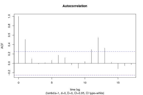
Title produced by software

(Partial) Autocorrelation Function

Date of computation

Fri, 03 Dec 2010 08:22:12 +0000

Cite this page as follows

Statistical Computations at FreeStatistics.org, Office for Research Development and Education, URL https://freestatistics.org/blog/index.php?v=date/2010/Dec/03/t12913644073i7q2ykhe4kws9l.htm/, Retrieved Tue, 07 May 2024 23:47:59 +0000

Statistical Computations at FreeStatistics.org, Office for Research Development and Education, URL https://freestatistics.org/blog/index.php?pk=104533, Retrieved Tue, 07 May 2024 23:47:59 +0000

QR Codes:

Paste this QR Code to cite your computation.

Original text written by user:

IsPrivate?

No (this computation is public)

User-defined keywords

Estimated Impact

154

Family? (F = Feedback message, R = changed R code, M = changed R Module, P = changed Parameters, D = changed Data)

-     [Univariate Data Series] [data set] [2008-12-01 19:54:57] [b98453cac15ba1066b407e146608df68]
- RMP   [(Partial) Autocorrelation Function] [Unemployment] [2010-11-29 09:05:21] [b98453cac15ba1066b407e146608df68]
-    D      [(Partial) Autocorrelation Function] [W9 autocorrelatie] [2010-12-03 08:22:12] [59f7d3e7fcb6374015f4e6b9053b0f01] [Current]
-             [(Partial) Autocorrelation Function] [W9 ACF] [2010-12-03 09:05:40] [56d90b683fcd93137645f9226b43c62b] 
-    D        [(Partial) Autocorrelation Function] [W9 ACF d=0 D=0] [2010-12-03 09:37:57] [56d90b683fcd93137645f9226b43c62b] 
-    D        [(Partial) Autocorrelation Function] [W9 ACF d=1 D=0] [2010-12-03 09:41:48] [56d90b683fcd93137645f9226b43c62b] 
-    D        [(Partial) Autocorrelation Function] [W9 d=1 D=1] [2010-12-03 09:48:24] [56d90b683fcd93137645f9226b43c62b] 

Feedback Forum

Post a new message

Dataseries X:

Download CSV

Histogram

Boxplots

Summary of computational transaction
Raw Input	view raw input (R code)
Raw Output	view raw output of R engine
Computing time	8 seconds
R Server	'George Udny Yule' @ 72.249.76.132

\begin{tabular}{lllllllll}
\hline
Summary of computational transaction \tabularnewline
Raw Input & view raw input (R code)  \tabularnewline
Raw Output & view raw output of R engine  \tabularnewline
Computing time & 8 seconds \tabularnewline
R Server & 'George Udny Yule' @ 72.249.76.132 \tabularnewline
\hline
\end{tabular}
%Source: https://freestatistics.org/blog/index.php?pk=104533&T=0

[TABLE]
[ROW][C]Summary of computational transaction[/C][/ROW]
[ROW][C]Raw Input[/C][C]view raw input (R code) [/C][/ROW]
[ROW][C]Raw Output[/C][C]view raw output of R engine [/C][/ROW]
[ROW][C]Computing time[/C][C]8 seconds[/C][/ROW]
[ROW][C]R Server[/C][C]'George Udny Yule' @ 72.249.76.132[/C][/ROW]
[/TABLE]
Source: https://freestatistics.org/blog/index.php?pk=104533&T=0

Globally Unique Identifier (entire table): ba.freestatistics.org/blog/index.php?pk=104533&T=0

As an alternative you can also use a QR Code:

The GUIDs for individual cells are displayed in the table below:

Summary of computational transaction
Raw Input	view raw input (R code)
Raw Output	view raw output of R engine
Computing time	8 seconds
R Server	'George Udny Yule' @ 72.249.76.132

Autocorrelation Function
Time lag k	ACF(k)	T-STAT	P-value
1	0.509969	3.9502	0.000104
2	0.097421	0.7546	0.226713
3	-0.012413	-0.0962	0.46186
4	0.015184	0.1176	0.453382
5	0.065753	0.5093	0.306198
6	0.175137	1.3566	0.089995
7	0.121471	0.9409	0.175261
8	-0.030507	-0.2363	0.406999
9	-0.104467	-0.8092	0.210799
10	0.04036	0.3126	0.377823
11	0.296111	2.2937	0.012664
12	0.548265	4.2468	3.8e-05
13	0.326629	2.5301	0.007024
14	0.023016	0.1783	0.429552
15	-0.1169	-0.9055	0.184411
16	-0.051444	-0.3985	0.345844
17	-0.029327	-0.2272	0.410532

\begin{tabular}{lllllllll}
\hline
Autocorrelation Function \tabularnewline
Time lag k & ACF(k) & T-STAT & P-value \tabularnewline
1 & 0.509969 & 3.9502 & 0.000104 \tabularnewline
2 & 0.097421 & 0.7546 & 0.226713 \tabularnewline
3 & -0.012413 & -0.0962 & 0.46186 \tabularnewline
4 & 0.015184 & 0.1176 & 0.453382 \tabularnewline
5 & 0.065753 & 0.5093 & 0.306198 \tabularnewline
6 & 0.175137 & 1.3566 & 0.089995 \tabularnewline
7 & 0.121471 & 0.9409 & 0.175261 \tabularnewline
8 & -0.030507 & -0.2363 & 0.406999 \tabularnewline
9 & -0.104467 & -0.8092 & 0.210799 \tabularnewline
10 & 0.04036 & 0.3126 & 0.377823 \tabularnewline
11 & 0.296111 & 2.2937 & 0.012664 \tabularnewline
12 & 0.548265 & 4.2468 & 3.8e-05 \tabularnewline
13 & 0.326629 & 2.5301 & 0.007024 \tabularnewline
14 & 0.023016 & 0.1783 & 0.429552 \tabularnewline
15 & -0.1169 & -0.9055 & 0.184411 \tabularnewline
16 & -0.051444 & -0.3985 & 0.345844 \tabularnewline
17 & -0.029327 & -0.2272 & 0.410532 \tabularnewline
\hline
\end{tabular}
%Source: https://freestatistics.org/blog/index.php?pk=104533&T=1

[TABLE]
[ROW][C]Autocorrelation Function[/C][/ROW]
[ROW][C]Time lag k[/C][C]ACF(k)[/C][C]T-STAT[/C][C]P-value[/C][/ROW]
[ROW][C]1[/C][C]0.509969[/C][C]3.9502[/C][C]0.000104[/C][/ROW]
[ROW][C]2[/C][C]0.097421[/C][C]0.7546[/C][C]0.226713[/C][/ROW]
[ROW][C]3[/C][C]-0.012413[/C][C]-0.0962[/C][C]0.46186[/C][/ROW]
[ROW][C]4[/C][C]0.015184[/C][C]0.1176[/C][C]0.453382[/C][/ROW]
[ROW][C]5[/C][C]0.065753[/C][C]0.5093[/C][C]0.306198[/C][/ROW]
[ROW][C]6[/C][C]0.175137[/C][C]1.3566[/C][C]0.089995[/C][/ROW]
[ROW][C]7[/C][C]0.121471[/C][C]0.9409[/C][C]0.175261[/C][/ROW]
[ROW][C]8[/C][C]-0.030507[/C][C]-0.2363[/C][C]0.406999[/C][/ROW]
[ROW][C]9[/C][C]-0.104467[/C][C]-0.8092[/C][C]0.210799[/C][/ROW]
[ROW][C]10[/C][C]0.04036[/C][C]0.3126[/C][C]0.377823[/C][/ROW]
[ROW][C]11[/C][C]0.296111[/C][C]2.2937[/C][C]0.012664[/C][/ROW]
[ROW][C]12[/C][C]0.548265[/C][C]4.2468[/C][C]3.8e-05[/C][/ROW]
[ROW][C]13[/C][C]0.326629[/C][C]2.5301[/C][C]0.007024[/C][/ROW]
[ROW][C]14[/C][C]0.023016[/C][C]0.1783[/C][C]0.429552[/C][/ROW]
[ROW][C]15[/C][C]-0.1169[/C][C]-0.9055[/C][C]0.184411[/C][/ROW]
[ROW][C]16[/C][C]-0.051444[/C][C]-0.3985[/C][C]0.345844[/C][/ROW]
[ROW][C]17[/C][C]-0.029327[/C][C]-0.2272[/C][C]0.410532[/C][/ROW]
[/TABLE]
Source: https://freestatistics.org/blog/index.php?pk=104533&T=1

Globally Unique Identifier (entire table): ba.freestatistics.org/blog/index.php?pk=104533&T=1

As an alternative you can also use a QR Code:

The GUIDs for individual cells are displayed in the table below:

Autocorrelation Function
Time lag k	ACF(k)	T-STAT	P-value
1	0.509969	3.9502	0.000104
2	0.097421	0.7546	0.226713
3	-0.012413	-0.0962	0.46186
4	0.015184	0.1176	0.453382
5	0.065753	0.5093	0.306198
6	0.175137	1.3566	0.089995
7	0.121471	0.9409	0.175261
8	-0.030507	-0.2363	0.406999
9	-0.104467	-0.8092	0.210799
10	0.04036	0.3126	0.377823
11	0.296111	2.2937	0.012664
12	0.548265	4.2468	3.8e-05
13	0.326629	2.5301	0.007024
14	0.023016	0.1783	0.429552
15	-0.1169	-0.9055	0.184411
16	-0.051444	-0.3985	0.345844
17	-0.029327	-0.2272	0.410532

Partial Autocorrelation Function
Time lag k	PACF(k)	T-STAT	P-value
1	0.509969	3.9502	0.000104
2	-0.219814	-1.7027	0.046903
3	0.055501	0.4299	0.334402
4	0.027823	0.2155	0.415048
5	0.05018	0.3887	0.349441
6	0.161247	1.249	0.108255
7	-0.071505	-0.5539	0.290862
8	-0.075846	-0.5875	0.279536
9	-0.032553	-0.2522	0.400892
10	0.161943	1.2544	0.10728
11	0.267647	2.0732	0.021229
12	0.382208	2.9606	0.002196
13	-0.183385	-1.4205	0.08032
14	-0.069067	-0.535	0.297317
15	-0.101108	-0.7832	0.2183
16	0.0412	0.3191	0.375367
17	-0.125131	-0.9693	0.168154

\begin{tabular}{lllllllll}
\hline
Partial Autocorrelation Function \tabularnewline
Time lag k & PACF(k) & T-STAT & P-value \tabularnewline
1 & 0.509969 & 3.9502 & 0.000104 \tabularnewline
2 & -0.219814 & -1.7027 & 0.046903 \tabularnewline
3 & 0.055501 & 0.4299 & 0.334402 \tabularnewline
4 & 0.027823 & 0.2155 & 0.415048 \tabularnewline
5 & 0.05018 & 0.3887 & 0.349441 \tabularnewline
6 & 0.161247 & 1.249 & 0.108255 \tabularnewline
7 & -0.071505 & -0.5539 & 0.290862 \tabularnewline
8 & -0.075846 & -0.5875 & 0.279536 \tabularnewline
9 & -0.032553 & -0.2522 & 0.400892 \tabularnewline
10 & 0.161943 & 1.2544 & 0.10728 \tabularnewline
11 & 0.267647 & 2.0732 & 0.021229 \tabularnewline
12 & 0.382208 & 2.9606 & 0.002196 \tabularnewline
13 & -0.183385 & -1.4205 & 0.08032 \tabularnewline
14 & -0.069067 & -0.535 & 0.297317 \tabularnewline
15 & -0.101108 & -0.7832 & 0.2183 \tabularnewline
16 & 0.0412 & 0.3191 & 0.375367 \tabularnewline
17 & -0.125131 & -0.9693 & 0.168154 \tabularnewline
\hline
\end{tabular}
%Source: https://freestatistics.org/blog/index.php?pk=104533&T=2

[TABLE]
[ROW][C]Partial Autocorrelation Function[/C][/ROW]
[ROW][C]Time lag k[/C][C]PACF(k)[/C][C]T-STAT[/C][C]P-value[/C][/ROW]
[ROW][C]1[/C][C]0.509969[/C][C]3.9502[/C][C]0.000104[/C][/ROW]
[ROW][C]2[/C][C]-0.219814[/C][C]-1.7027[/C][C]0.046903[/C][/ROW]
[ROW][C]3[/C][C]0.055501[/C][C]0.4299[/C][C]0.334402[/C][/ROW]
[ROW][C]4[/C][C]0.027823[/C][C]0.2155[/C][C]0.415048[/C][/ROW]
[ROW][C]5[/C][C]0.05018[/C][C]0.3887[/C][C]0.349441[/C][/ROW]
[ROW][C]6[/C][C]0.161247[/C][C]1.249[/C][C]0.108255[/C][/ROW]
[ROW][C]7[/C][C]-0.071505[/C][C]-0.5539[/C][C]0.290862[/C][/ROW]
[ROW][C]8[/C][C]-0.075846[/C][C]-0.5875[/C][C]0.279536[/C][/ROW]
[ROW][C]9[/C][C]-0.032553[/C][C]-0.2522[/C][C]0.400892[/C][/ROW]
[ROW][C]10[/C][C]0.161943[/C][C]1.2544[/C][C]0.10728[/C][/ROW]
[ROW][C]11[/C][C]0.267647[/C][C]2.0732[/C][C]0.021229[/C][/ROW]
[ROW][C]12[/C][C]0.382208[/C][C]2.9606[/C][C]0.002196[/C][/ROW]
[ROW][C]13[/C][C]-0.183385[/C][C]-1.4205[/C][C]0.08032[/C][/ROW]
[ROW][C]14[/C][C]-0.069067[/C][C]-0.535[/C][C]0.297317[/C][/ROW]
[ROW][C]15[/C][C]-0.101108[/C][C]-0.7832[/C][C]0.2183[/C][/ROW]
[ROW][C]16[/C][C]0.0412[/C][C]0.3191[/C][C]0.375367[/C][/ROW]
[ROW][C]17[/C][C]-0.125131[/C][C]-0.9693[/C][C]0.168154[/C][/ROW]
[/TABLE]
Source: https://freestatistics.org/blog/index.php?pk=104533&T=2

Globally Unique Identifier (entire table): ba.freestatistics.org/blog/index.php?pk=104533&T=2

As an alternative you can also use a QR Code:

The GUIDs for individual cells are displayed in the table below:

Partial Autocorrelation Function
Time lag k	PACF(k)	T-STAT	P-value
1	0.509969	3.9502	0.000104
2	-0.219814	-1.7027	0.046903
3	0.055501	0.4299	0.334402
4	0.027823	0.2155	0.415048
5	0.05018	0.3887	0.349441
6	0.161247	1.249	0.108255
7	-0.071505	-0.5539	0.290862
8	-0.075846	-0.5875	0.279536
9	-0.032553	-0.2522	0.400892
10	0.161943	1.2544	0.10728
11	0.267647	2.0732	0.021229
12	0.382208	2.9606	0.002196
13	-0.183385	-1.4205	0.08032
14	-0.069067	-0.535	0.297317
15	-0.101108	-0.7832	0.2183
16	0.0412	0.3191	0.375367
17	-0.125131	-0.9693	0.168154

Figure 1

PNG link

Postscript link

PDF link

Figure 2

PNG link

Postscript link

PDF link

Parameters (Session):

par1 = Default ; par2 = 1 ; par3 = 0 ; par4 = 0 ; par5 = 12 ; par6 = White Noise ; par7 = 0.95 ;

Parameters (R input):

par1 = Default ; par2 = 1 ; par3 = 0 ; par4 = 0 ; par5 = 12 ; par6 = White Noise ; par7 = 0.95 ;

R code (references can be found in the software module):

if (par1 == 'Default') {
par1 = 10*log10(length(x))
} else {
par1 <- as.numeric(par1)
}
par2 <- as.numeric(par2)
par3 <- as.numeric(par3)
par4 <- as.numeric(par4)
par5 <- as.numeric(par5)
if (par6 == 'White Noise') par6 <- 'white' else par6 <- 'ma'
par7 <- as.numeric(par7)
if (par2 == 0) {
x <- log(x)
} else {
x <- (x ^ par2 - 1) / par2
}
if (par3 > 0) x <- diff(x,lag=1,difference=par3)
if (par4 > 0) x <- diff(x,lag=par5,difference=par4)
bitmap(file='pic1.png')
racf <- acf(x, par1, main='Autocorrelation', xlab='time lag', ylab='ACF', ci.type=par6, ci=par7, sub=paste('(lambda=',par2,', d=',par3,', D=',par4,', CI=', par7, ', CI type=',par6,')',sep=''))
dev.off()
bitmap(file='pic2.png')
rpacf <- pacf(x,par1,main='Partial Autocorrelation',xlab='lags',ylab='PACF')
dev.off()
(myacf <- c(racf$acf))
(mypacf <- c(rpacf$acf))
lengthx <- length(x)
sqrtn <- sqrt(lengthx)
load(file='createtable')
a<-table.start()
a<-table.row.start(a)
a<-table.element(a,'Autocorrelation Function',4,TRUE)
a<-table.row.end(a)
a<-table.row.start(a)
a<-table.element(a,'Time lag k',header=TRUE)
a<-table.element(a,hyperlink('basics.htm','ACF(k)','click here for more information about the Autocorrelation Function'),header=TRUE)
a<-table.element(a,'T-STAT',header=TRUE)
a<-table.element(a,'P-value',header=TRUE)
a<-table.row.end(a)
for (i in 2:(par1+1)) {
a<-table.row.start(a)
a<-table.element(a,i-1,header=TRUE)
a<-table.element(a,round(myacf[i],6))
mytstat <- myacf[i]*sqrtn
a<-table.element(a,round(mytstat,4))
a<-table.element(a,round(1-pt(abs(mytstat),lengthx),6))
a<-table.row.end(a)
}
a<-table.end(a)
table.save(a,file='mytable.tab')
a<-table.start()
a<-table.row.start(a)
a<-table.element(a,'Partial Autocorrelation Function',4,TRUE)
a<-table.row.end(a)
a<-table.row.start(a)
a<-table.element(a,'Time lag k',header=TRUE)
a<-table.element(a,hyperlink('basics.htm','PACF(k)','click here for more information about the Partial Autocorrelation Function'),header=TRUE)
a<-table.element(a,'T-STAT',header=TRUE)
a<-table.element(a,'P-value',header=TRUE)
a<-table.row.end(a)
for (i in 1:par1) {
a<-table.row.start(a)
a<-table.element(a,i,header=TRUE)
a<-table.element(a,round(mypacf[i],6))
mytstat <- mypacf[i]*sqrtn
a<-table.element(a,round(mytstat,4))
a<-table.element(a,round(1-pt(abs(mytstat),lengthx),6))
a<-table.row.end(a)
}
a<-table.end(a)
table.save(a,file='mytable1.tab')

Free Statistics

Description of Statistical Computation

Tree of Dependent Computations

Dataset

Tables (Output of Computation)

Figures (Output of Computation)

Input Parameters & R Code