Free Statistics
of Irreproducible Research!
Description of Statistical Computation | |||||||||||||||||||||
|---|---|---|---|---|---|---|---|---|---|---|---|---|---|---|---|---|---|---|---|---|---|
| Author's title | |||||||||||||||||||||
| Author | *Unverified author* | ||||||||||||||||||||
| R Software Module | rwasp_meanplot.wasp | ||||||||||||||||||||
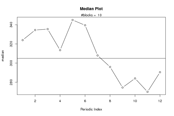
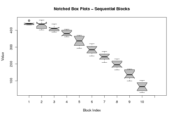
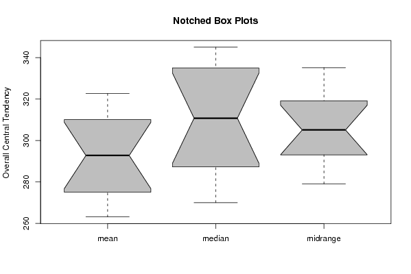
| Title produced by software | Mean Plot | ||||||||||||||||||||
| Date of computation | Mon, 02 Aug 2010 11:28:43 +0000 | ||||||||||||||||||||
| Cite this page as follows | Statistical Computations at FreeStatistics.org, Office for Research Development and Education, URL https://freestatistics.org/blog/index.php?v=date/2010/Aug/02/t12807499084xcxlpigosvv7nl.htm/, Retrieved Wed, 01 May 2024 23:47:41 +0000 | ||||||||||||||||||||
| Statistical Computations at FreeStatistics.org, Office for Research Development and Education, URL https://freestatistics.org/blog/index.php?pk=78215, Retrieved Wed, 01 May 2024 23:47:41 +0000 | |||||||||||||||||||||
| QR Codes: | |||||||||||||||||||||
|
| |||||||||||||||||||||
| Original text written by user: | |||||||||||||||||||||
| IsPrivate? | No (this computation is public) | ||||||||||||||||||||
| User-defined keywords | Bogaerts Yannik | ||||||||||||||||||||
| Estimated Impact | 208 | ||||||||||||||||||||
Tree of Dependent Computations | |||||||||||||||||||||
| Family? (F = Feedback message, R = changed R code, M = changed R Module, P = changed Parameters, D = changed Data) | |||||||||||||||||||||
| - [Harrell-Davis Quantiles] [Tijdreeks A stap 11] [2010-08-02 10:14:58] [f713c1ac4846c73da8c41c71cf7e0185] - RMP [Mean Plot] [Tijdreeks A stap 17] [2010-08-02 11:28:43] [1596366c2ece8f787477cc7d1246d4c7] [Current] | |||||||||||||||||||||
| Feedback Forum | |||||||||||||||||||||
Post a new message | |||||||||||||||||||||
Dataset | |||||||||||||||||||||
| Dataseries X: | |||||||||||||||||||||
442 441 440 438 458 457 442 432 433 433 434 436 439 439 441 436 460 453 435 421 412 408 402 409 410 410 416 410 437 431 411 398 394 395 389 404 397 401 402 383 406 400 377 372 362 365 361 372 355 365 367 341 370 366 333 320 298 306 293 313 293 304 304 286 320 313 283 272 251 262 247 268 251 257 261 242 274 272 243 234 217 231 209 226 208 214 222 194 230 226 197 188 175 190 165 176 159 169 170 141 170 164 132 123 113 125 101 99 87 90 89 66 102 97 65 54 33 49 30 34 | |||||||||||||||||||||
Tables (Output of Computation) | |||||||||||||||||||||
| |||||||||||||||||||||
Figures (Output of Computation) | |||||||||||||||||||||
Input Parameters & R Code | |||||||||||||||||||||
| Parameters (Session): | |||||||||||||||||||||
| par1 = 12 ; | |||||||||||||||||||||
| Parameters (R input): | |||||||||||||||||||||
| par1 = 12 ; | |||||||||||||||||||||
| R code (references can be found in the software module): | |||||||||||||||||||||
par1 <- as.numeric(par1) | |||||||||||||||||||||