Free Statistics
of Irreproducible Research!
Description of Statistical Computation | |||||||||||||||||||||||||||||||||||||||||||||||||||||||||||||||||||||||||||||||||
|---|---|---|---|---|---|---|---|---|---|---|---|---|---|---|---|---|---|---|---|---|---|---|---|---|---|---|---|---|---|---|---|---|---|---|---|---|---|---|---|---|---|---|---|---|---|---|---|---|---|---|---|---|---|---|---|---|---|---|---|---|---|---|---|---|---|---|---|---|---|---|---|---|---|---|---|---|---|---|---|---|---|
| Author's title | |||||||||||||||||||||||||||||||||||||||||||||||||||||||||||||||||||||||||||||||||
| Author | *Unverified author* | ||||||||||||||||||||||||||||||||||||||||||||||||||||||||||||||||||||||||||||||||
| R Software Module | rwasp_bootstrapplot1.wasp | ||||||||||||||||||||||||||||||||||||||||||||||||||||||||||||||||||||||||||||||||
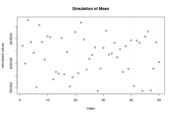
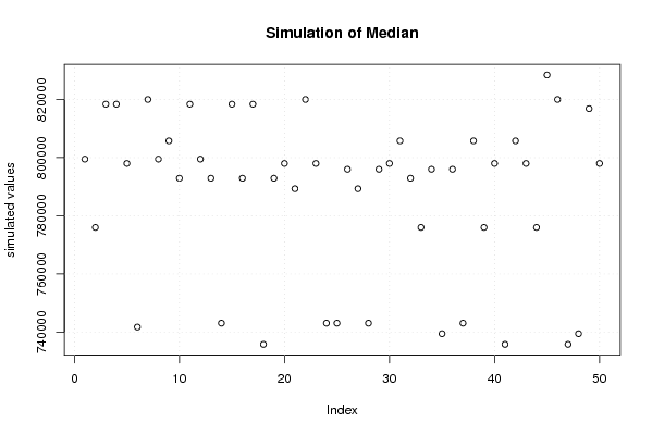
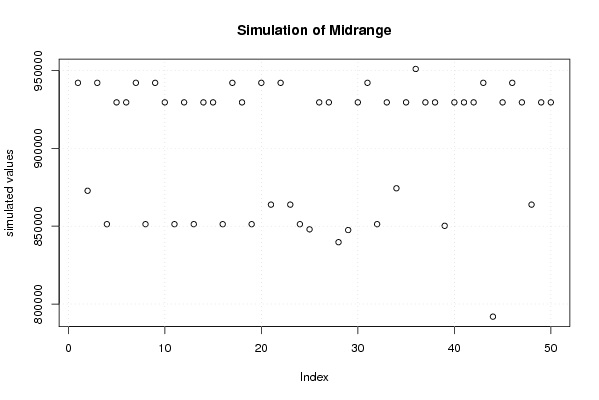
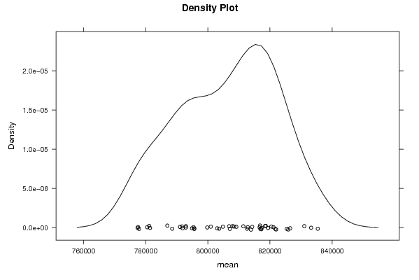
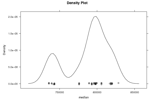
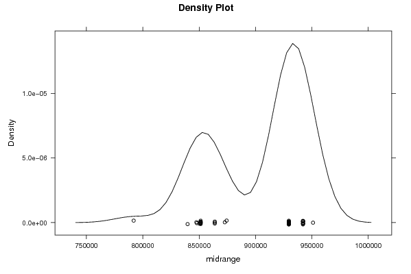
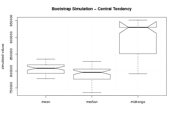
| Title produced by software | Bootstrap Plot - Central Tendency | ||||||||||||||||||||||||||||||||||||||||||||||||||||||||||||||||||||||||||||||||
| Date of computation | Thu, 04 Jun 2009 09:33:12 -0600 | ||||||||||||||||||||||||||||||||||||||||||||||||||||||||||||||||||||||||||||||||
| Cite this page as follows | Statistical Computations at FreeStatistics.org, Office for Research Development and Education, URL https://freestatistics.org/blog/index.php?v=date/2009/Jun/04/t1244129621dnhptoxjyc8mcgc.htm/, Retrieved Tue, 01 Jul 2025 00:38:47 +0000 | ||||||||||||||||||||||||||||||||||||||||||||||||||||||||||||||||||||||||||||||||
| Statistical Computations at FreeStatistics.org, Office for Research Development and Education, URL https://freestatistics.org/blog/index.php?pk=41710, Retrieved Tue, 01 Jul 2025 00:38:47 +0000 | |||||||||||||||||||||||||||||||||||||||||||||||||||||||||||||||||||||||||||||||||
| QR Codes: | |||||||||||||||||||||||||||||||||||||||||||||||||||||||||||||||||||||||||||||||||
|
| |||||||||||||||||||||||||||||||||||||||||||||||||||||||||||||||||||||||||||||||||
| Original text written by user: | |||||||||||||||||||||||||||||||||||||||||||||||||||||||||||||||||||||||||||||||||
| IsPrivate? | No (this computation is public) | ||||||||||||||||||||||||||||||||||||||||||||||||||||||||||||||||||||||||||||||||
| User-defined keywords | |||||||||||||||||||||||||||||||||||||||||||||||||||||||||||||||||||||||||||||||||
| Estimated Impact | 151 | ||||||||||||||||||||||||||||||||||||||||||||||||||||||||||||||||||||||||||||||||
Tree of Dependent Computations | |||||||||||||||||||||||||||||||||||||||||||||||||||||||||||||||||||||||||||||||||
| Family? (F = Feedback message, R = changed R code, M = changed R Module, P = changed Parameters, D = changed Data) | |||||||||||||||||||||||||||||||||||||||||||||||||||||||||||||||||||||||||||||||||
| - [Bootstrap Plot - Central Tendency] [bootstrapplot] [2009-06-04 15:33:12] [d41d8cd98f00b204e9800998ecf8427e] [Current] - D [Bootstrap Plot - Central Tendency] [opgave 7 dennis gys] [2009-06-05 13:31:33] [74be16979710d4c4e7c6647856088456] - RMPD [Classical Decomposition] [opgave9W.Verlinden] [2009-06-05 13:55:11] [74be16979710d4c4e7c6647856088456] - [Classical Decomposition] [opgave 9 Dennis Gys] [2009-06-06 11:11:29] [74be16979710d4c4e7c6647856088456] - D [Classical Decomposition] [opgave 9(2) denni...] [2009-06-06 11:16:53] [74be16979710d4c4e7c6647856088456] - PD [Bootstrap Plot - Central Tendency] [opgave 7(2) denni...] [2009-06-05 13:56:25] [74be16979710d4c4e7c6647856088456] - RMP [Classical Decomposition] [opgave9bW.Verlinden] [2009-06-05 14:07:30] [74be16979710d4c4e7c6647856088456] - RMPD [Exponential Smoothing] [opgave10W.Verlinden] [2009-06-05 15:07:33] [74be16979710d4c4e7c6647856088456] - [Exponential Smoothing] [opgave 10 dennis gys] [2009-06-06 11:28:51] [74be16979710d4c4e7c6647856088456] - D [Exponential Smoothing] [opgave 10(2) denn...] [2009-06-06 11:35:11] [74be16979710d4c4e7c6647856088456] - RMP [Exponential Smoothing] [opgave10bW.Verlinden] [2009-06-05 15:15:35] [74be16979710d4c4e7c6647856088456] | |||||||||||||||||||||||||||||||||||||||||||||||||||||||||||||||||||||||||||||||||
| Feedback Forum | |||||||||||||||||||||||||||||||||||||||||||||||||||||||||||||||||||||||||||||||||
Post a new message | |||||||||||||||||||||||||||||||||||||||||||||||||||||||||||||||||||||||||||||||||
Dataset | |||||||||||||||||||||||||||||||||||||||||||||||||||||||||||||||||||||||||||||||||
| Dataseries X: | |||||||||||||||||||||||||||||||||||||||||||||||||||||||||||||||||||||||||||||||||
665272 661735 621014 574889 677734 717075 653612 690697 665864 830701 789303 617808 805775 909449 599973 955874 799494 876097 823300 900079 860754 923882 1121084 741757 966066 901978 648659 852732 706036 835792 722489 714262 739459 816834 743082 683375 1006000 866000 644000 703000 699000 713000 688000 672000 600000 847000 697000 687000 973000 796000 658000 709000 798000 820000 776000 699000 828433 942131 792916 864942 982689 948143 874863 735794 854605 1284216 961585 818379 1079498 1095091 1008925 967118 1127715 | |||||||||||||||||||||||||||||||||||||||||||||||||||||||||||||||||||||||||||||||||
Tables (Output of Computation) | |||||||||||||||||||||||||||||||||||||||||||||||||||||||||||||||||||||||||||||||||
| |||||||||||||||||||||||||||||||||||||||||||||||||||||||||||||||||||||||||||||||||
Figures (Output of Computation) | |||||||||||||||||||||||||||||||||||||||||||||||||||||||||||||||||||||||||||||||||
Input Parameters & R Code | |||||||||||||||||||||||||||||||||||||||||||||||||||||||||||||||||||||||||||||||||
| Parameters (Session): | |||||||||||||||||||||||||||||||||||||||||||||||||||||||||||||||||||||||||||||||||
| par1 = 50 ; | |||||||||||||||||||||||||||||||||||||||||||||||||||||||||||||||||||||||||||||||||
| Parameters (R input): | |||||||||||||||||||||||||||||||||||||||||||||||||||||||||||||||||||||||||||||||||
| par1 = 50 ; | |||||||||||||||||||||||||||||||||||||||||||||||||||||||||||||||||||||||||||||||||
| R code (references can be found in the software module): | |||||||||||||||||||||||||||||||||||||||||||||||||||||||||||||||||||||||||||||||||
par1 <- as.numeric(par1) | |||||||||||||||||||||||||||||||||||||||||||||||||||||||||||||||||||||||||||||||||