Repository of Reproducible Computations

Free Statistics

of Irreproducible Research!

Author's title

Author

*Unverified author*

R Software Module

rwasp_autocorrelation.wasp

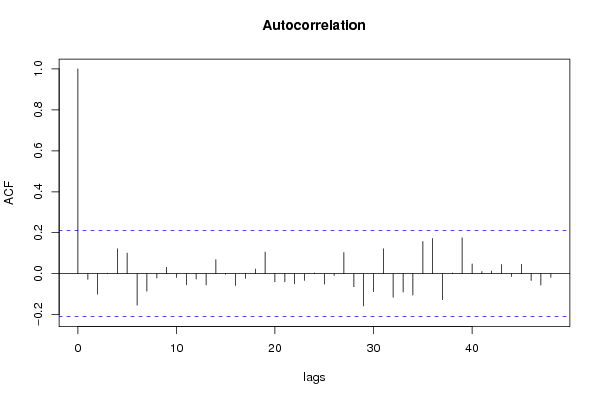
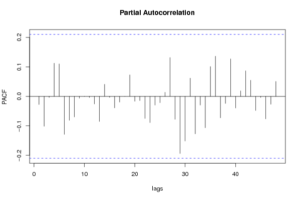
Title produced by software

(Partial) Autocorrelation Function

Date of computation

Thu, 04 Jun 2009 09:02:05 -0600

Cite this page as follows

Statistical Computations at FreeStatistics.org, Office for Research Development and Education, URL https://freestatistics.org/blog/index.php?v=date/2009/Jun/04/t1244127963wou9tyyktpagtqe.htm/, Retrieved Tue, 14 May 2024 00:42:41 +0000

Statistical Computations at FreeStatistics.org, Office for Research Development and Education, URL https://freestatistics.org/blog/index.php?pk=41705, Retrieved Tue, 14 May 2024 00:42:41 +0000

QR Codes:

Paste this QR Code to cite your computation.

Original text written by user:

IsPrivate?

No (this computation is public)

User-defined keywords

Estimated Impact

106

Family? (F = Feedback message, R = changed R code, M = changed R Module, P = changed Parameters, D = changed Data)

-       [(Partial) Autocorrelation Function] [opgave6bisoef2stap2] [2009-06-04 15:02:05] [791ed687546d9528c8a01d986e6abead] [Current]

Feedback Forum

Post a new message

Dataseries X:

Download CSV

Histogram

Boxplots

Summary of computational transaction
Raw Input	view raw input (R code)
Raw Output	view raw output of R engine
Computing time	1 seconds
R Server	'Gwilym Jenkins' @ 72.249.127.135

\begin{tabular}{lllllllll}
\hline
Summary of computational transaction \tabularnewline
Raw Input & view raw input (R code)  \tabularnewline
Raw Output & view raw output of R engine  \tabularnewline
Computing time & 1 seconds \tabularnewline
R Server & 'Gwilym Jenkins' @ 72.249.127.135 \tabularnewline
\hline
\end{tabular}
%Source: https://freestatistics.org/blog/index.php?pk=41705&T=0

[TABLE]
[ROW][C]Summary of computational transaction[/C][/ROW]
[ROW][C]Raw Input[/C][C]view raw input (R code) [/C][/ROW]
[ROW][C]Raw Output[/C][C]view raw output of R engine [/C][/ROW]
[ROW][C]Computing time[/C][C]1 seconds[/C][/ROW]
[ROW][C]R Server[/C][C]'Gwilym Jenkins' @ 72.249.127.135[/C][/ROW]
[/TABLE]
Source: https://freestatistics.org/blog/index.php?pk=41705&T=0

Globally Unique Identifier (entire table): ba.freestatistics.org/blog/index.php?pk=41705&T=0

As an alternative you can also use a QR Code:

The GUIDs for individual cells are displayed in the table below:

Summary of computational transaction
Raw Input	view raw input (R code)
Raw Output	view raw output of R engine
Computing time	1 seconds
R Server	'Gwilym Jenkins' @ 72.249.127.135

Autocorrelation Function
Time lag k	ACF(k)	T-STAT	P-value
1	-0.027566	-0.2571	0.398847
2	-0.100478	-0.9372	0.175626
3	0.002328	0.0217	0.491363
4	0.12161	1.1343	0.129892
5	0.1007	0.9393	0.175098
6	-0.154222	-1.4385	0.076942
7	-0.085664	-0.799	0.213227
8	-0.021765	-0.203	0.419802
9	0.031052	0.2896	0.386394
10	-0.01825	-0.1702	0.432613
11	-0.054344	-0.5069	0.306758
12	-0.026621	-0.2483	0.402241
13	-0.055389	-0.5166	0.303362
14	0.06831	0.6372	0.26285
15	-0.003071	-0.0286	0.488609
16	-0.057693	-0.5381	0.295933
17	-0.02279	-0.2126	0.416079
18	0.022686	0.2116	0.416457
19	0.105395	0.9831	0.164152
20	-0.039059	-0.3643	0.358251
21	-0.03983	-0.3715	0.355582
22	-0.049906	-0.4655	0.32137
23	-0.033255	-0.3102	0.378582
24	0.003012	0.0281	0.488825
25	-0.050731	-0.4732	0.318633
26	-0.008832	-0.0824	0.467265
27	0.10326	0.9631	0.169072
28	-0.063488	-0.5922	0.277633
29	-0.157487	-1.4689	0.072727
30	-0.08833	-0.8239	0.206129
31	0.12122	1.1307	0.130652
32	-0.115663	-1.0788	0.141822
33	-0.090156	-0.8409	0.20135
34	-0.10489	-0.9783	0.165308
35	0.157459	1.4687	0.072763
36	0.172043	1.6047	0.056091
37	-0.127098	-1.1855	0.119526
38	0.002593	0.0242	0.490378
39	0.174876	1.6311	0.053238
40	0.047195	0.4402	0.33044
41	0.01041	0.0971	0.461436
42	0.012705	0.1185	0.452971
43	0.044143	0.4117	0.340771
44	-0.014051	-0.1311	0.448016
45	0.045778	0.427	0.33522
46	-0.033186	-0.3095	0.378825
47	-0.055524	-0.5179	0.302922
48	-0.017665	-0.1648	0.434754

\begin{tabular}{lllllllll}
\hline
Autocorrelation Function \tabularnewline
Time lag k & ACF(k) & T-STAT & P-value \tabularnewline
1 & -0.027566 & -0.2571 & 0.398847 \tabularnewline
2 & -0.100478 & -0.9372 & 0.175626 \tabularnewline
3 & 0.002328 & 0.0217 & 0.491363 \tabularnewline
4 & 0.12161 & 1.1343 & 0.129892 \tabularnewline
5 & 0.1007 & 0.9393 & 0.175098 \tabularnewline
6 & -0.154222 & -1.4385 & 0.076942 \tabularnewline
7 & -0.085664 & -0.799 & 0.213227 \tabularnewline
8 & -0.021765 & -0.203 & 0.419802 \tabularnewline
9 & 0.031052 & 0.2896 & 0.386394 \tabularnewline
10 & -0.01825 & -0.1702 & 0.432613 \tabularnewline
11 & -0.054344 & -0.5069 & 0.306758 \tabularnewline
12 & -0.026621 & -0.2483 & 0.402241 \tabularnewline
13 & -0.055389 & -0.5166 & 0.303362 \tabularnewline
14 & 0.06831 & 0.6372 & 0.26285 \tabularnewline
15 & -0.003071 & -0.0286 & 0.488609 \tabularnewline
16 & -0.057693 & -0.5381 & 0.295933 \tabularnewline
17 & -0.02279 & -0.2126 & 0.416079 \tabularnewline
18 & 0.022686 & 0.2116 & 0.416457 \tabularnewline
19 & 0.105395 & 0.9831 & 0.164152 \tabularnewline
20 & -0.039059 & -0.3643 & 0.358251 \tabularnewline
21 & -0.03983 & -0.3715 & 0.355582 \tabularnewline
22 & -0.049906 & -0.4655 & 0.32137 \tabularnewline
23 & -0.033255 & -0.3102 & 0.378582 \tabularnewline
24 & 0.003012 & 0.0281 & 0.488825 \tabularnewline
25 & -0.050731 & -0.4732 & 0.318633 \tabularnewline
26 & -0.008832 & -0.0824 & 0.467265 \tabularnewline
27 & 0.10326 & 0.9631 & 0.169072 \tabularnewline
28 & -0.063488 & -0.5922 & 0.277633 \tabularnewline
29 & -0.157487 & -1.4689 & 0.072727 \tabularnewline
30 & -0.08833 & -0.8239 & 0.206129 \tabularnewline
31 & 0.12122 & 1.1307 & 0.130652 \tabularnewline
32 & -0.115663 & -1.0788 & 0.141822 \tabularnewline
33 & -0.090156 & -0.8409 & 0.20135 \tabularnewline
34 & -0.10489 & -0.9783 & 0.165308 \tabularnewline
35 & 0.157459 & 1.4687 & 0.072763 \tabularnewline
36 & 0.172043 & 1.6047 & 0.056091 \tabularnewline
37 & -0.127098 & -1.1855 & 0.119526 \tabularnewline
38 & 0.002593 & 0.0242 & 0.490378 \tabularnewline
39 & 0.174876 & 1.6311 & 0.053238 \tabularnewline
40 & 0.047195 & 0.4402 & 0.33044 \tabularnewline
41 & 0.01041 & 0.0971 & 0.461436 \tabularnewline
42 & 0.012705 & 0.1185 & 0.452971 \tabularnewline
43 & 0.044143 & 0.4117 & 0.340771 \tabularnewline
44 & -0.014051 & -0.1311 & 0.448016 \tabularnewline
45 & 0.045778 & 0.427 & 0.33522 \tabularnewline
46 & -0.033186 & -0.3095 & 0.378825 \tabularnewline
47 & -0.055524 & -0.5179 & 0.302922 \tabularnewline
48 & -0.017665 & -0.1648 & 0.434754 \tabularnewline
\hline
\end{tabular}
%Source: https://freestatistics.org/blog/index.php?pk=41705&T=1

[TABLE]
[ROW][C]Autocorrelation Function[/C][/ROW]
[ROW][C]Time lag k[/C][C]ACF(k)[/C][C]T-STAT[/C][C]P-value[/C][/ROW]
[ROW][C]1[/C][C]-0.027566[/C][C]-0.2571[/C][C]0.398847[/C][/ROW]
[ROW][C]2[/C][C]-0.100478[/C][C]-0.9372[/C][C]0.175626[/C][/ROW]
[ROW][C]3[/C][C]0.002328[/C][C]0.0217[/C][C]0.491363[/C][/ROW]
[ROW][C]4[/C][C]0.12161[/C][C]1.1343[/C][C]0.129892[/C][/ROW]
[ROW][C]5[/C][C]0.1007[/C][C]0.9393[/C][C]0.175098[/C][/ROW]
[ROW][C]6[/C][C]-0.154222[/C][C]-1.4385[/C][C]0.076942[/C][/ROW]
[ROW][C]7[/C][C]-0.085664[/C][C]-0.799[/C][C]0.213227[/C][/ROW]
[ROW][C]8[/C][C]-0.021765[/C][C]-0.203[/C][C]0.419802[/C][/ROW]
[ROW][C]9[/C][C]0.031052[/C][C]0.2896[/C][C]0.386394[/C][/ROW]
[ROW][C]10[/C][C]-0.01825[/C][C]-0.1702[/C][C]0.432613[/C][/ROW]
[ROW][C]11[/C][C]-0.054344[/C][C]-0.5069[/C][C]0.306758[/C][/ROW]
[ROW][C]12[/C][C]-0.026621[/C][C]-0.2483[/C][C]0.402241[/C][/ROW]
[ROW][C]13[/C][C]-0.055389[/C][C]-0.5166[/C][C]0.303362[/C][/ROW]
[ROW][C]14[/C][C]0.06831[/C][C]0.6372[/C][C]0.26285[/C][/ROW]
[ROW][C]15[/C][C]-0.003071[/C][C]-0.0286[/C][C]0.488609[/C][/ROW]
[ROW][C]16[/C][C]-0.057693[/C][C]-0.5381[/C][C]0.295933[/C][/ROW]
[ROW][C]17[/C][C]-0.02279[/C][C]-0.2126[/C][C]0.416079[/C][/ROW]
[ROW][C]18[/C][C]0.022686[/C][C]0.2116[/C][C]0.416457[/C][/ROW]
[ROW][C]19[/C][C]0.105395[/C][C]0.9831[/C][C]0.164152[/C][/ROW]
[ROW][C]20[/C][C]-0.039059[/C][C]-0.3643[/C][C]0.358251[/C][/ROW]
[ROW][C]21[/C][C]-0.03983[/C][C]-0.3715[/C][C]0.355582[/C][/ROW]
[ROW][C]22[/C][C]-0.049906[/C][C]-0.4655[/C][C]0.32137[/C][/ROW]
[ROW][C]23[/C][C]-0.033255[/C][C]-0.3102[/C][C]0.378582[/C][/ROW]
[ROW][C]24[/C][C]0.003012[/C][C]0.0281[/C][C]0.488825[/C][/ROW]
[ROW][C]25[/C][C]-0.050731[/C][C]-0.4732[/C][C]0.318633[/C][/ROW]
[ROW][C]26[/C][C]-0.008832[/C][C]-0.0824[/C][C]0.467265[/C][/ROW]
[ROW][C]27[/C][C]0.10326[/C][C]0.9631[/C][C]0.169072[/C][/ROW]
[ROW][C]28[/C][C]-0.063488[/C][C]-0.5922[/C][C]0.277633[/C][/ROW]
[ROW][C]29[/C][C]-0.157487[/C][C]-1.4689[/C][C]0.072727[/C][/ROW]
[ROW][C]30[/C][C]-0.08833[/C][C]-0.8239[/C][C]0.206129[/C][/ROW]
[ROW][C]31[/C][C]0.12122[/C][C]1.1307[/C][C]0.130652[/C][/ROW]
[ROW][C]32[/C][C]-0.115663[/C][C]-1.0788[/C][C]0.141822[/C][/ROW]
[ROW][C]33[/C][C]-0.090156[/C][C]-0.8409[/C][C]0.20135[/C][/ROW]
[ROW][C]34[/C][C]-0.10489[/C][C]-0.9783[/C][C]0.165308[/C][/ROW]
[ROW][C]35[/C][C]0.157459[/C][C]1.4687[/C][C]0.072763[/C][/ROW]
[ROW][C]36[/C][C]0.172043[/C][C]1.6047[/C][C]0.056091[/C][/ROW]
[ROW][C]37[/C][C]-0.127098[/C][C]-1.1855[/C][C]0.119526[/C][/ROW]
[ROW][C]38[/C][C]0.002593[/C][C]0.0242[/C][C]0.490378[/C][/ROW]
[ROW][C]39[/C][C]0.174876[/C][C]1.6311[/C][C]0.053238[/C][/ROW]
[ROW][C]40[/C][C]0.047195[/C][C]0.4402[/C][C]0.33044[/C][/ROW]
[ROW][C]41[/C][C]0.01041[/C][C]0.0971[/C][C]0.461436[/C][/ROW]
[ROW][C]42[/C][C]0.012705[/C][C]0.1185[/C][C]0.452971[/C][/ROW]
[ROW][C]43[/C][C]0.044143[/C][C]0.4117[/C][C]0.340771[/C][/ROW]
[ROW][C]44[/C][C]-0.014051[/C][C]-0.1311[/C][C]0.448016[/C][/ROW]
[ROW][C]45[/C][C]0.045778[/C][C]0.427[/C][C]0.33522[/C][/ROW]
[ROW][C]46[/C][C]-0.033186[/C][C]-0.3095[/C][C]0.378825[/C][/ROW]
[ROW][C]47[/C][C]-0.055524[/C][C]-0.5179[/C][C]0.302922[/C][/ROW]
[ROW][C]48[/C][C]-0.017665[/C][C]-0.1648[/C][C]0.434754[/C][/ROW]
[/TABLE]
Source: https://freestatistics.org/blog/index.php?pk=41705&T=1

Globally Unique Identifier (entire table): ba.freestatistics.org/blog/index.php?pk=41705&T=1

As an alternative you can also use a QR Code:

The GUIDs for individual cells are displayed in the table below:

Autocorrelation Function
Time lag k	ACF(k)	T-STAT	P-value
1	-0.027566	-0.2571	0.398847
2	-0.100478	-0.9372	0.175626
3	0.002328	0.0217	0.491363
4	0.12161	1.1343	0.129892
5	0.1007	0.9393	0.175098
6	-0.154222	-1.4385	0.076942
7	-0.085664	-0.799	0.213227
8	-0.021765	-0.203	0.419802
9	0.031052	0.2896	0.386394
10	-0.01825	-0.1702	0.432613
11	-0.054344	-0.5069	0.306758
12	-0.026621	-0.2483	0.402241
13	-0.055389	-0.5166	0.303362
14	0.06831	0.6372	0.26285
15	-0.003071	-0.0286	0.488609
16	-0.057693	-0.5381	0.295933
17	-0.02279	-0.2126	0.416079
18	0.022686	0.2116	0.416457
19	0.105395	0.9831	0.164152
20	-0.039059	-0.3643	0.358251
21	-0.03983	-0.3715	0.355582
22	-0.049906	-0.4655	0.32137
23	-0.033255	-0.3102	0.378582
24	0.003012	0.0281	0.488825
25	-0.050731	-0.4732	0.318633
26	-0.008832	-0.0824	0.467265
27	0.10326	0.9631	0.169072
28	-0.063488	-0.5922	0.277633
29	-0.157487	-1.4689	0.072727
30	-0.08833	-0.8239	0.206129
31	0.12122	1.1307	0.130652
32	-0.115663	-1.0788	0.141822
33	-0.090156	-0.8409	0.20135
34	-0.10489	-0.9783	0.165308
35	0.157459	1.4687	0.072763
36	0.172043	1.6047	0.056091
37	-0.127098	-1.1855	0.119526
38	0.002593	0.0242	0.490378
39	0.174876	1.6311	0.053238
40	0.047195	0.4402	0.33044
41	0.01041	0.0971	0.461436
42	0.012705	0.1185	0.452971
43	0.044143	0.4117	0.340771
44	-0.014051	-0.1311	0.448016
45	0.045778	0.427	0.33522
46	-0.033186	-0.3095	0.378825
47	-0.055524	-0.5179	0.302922
48	-0.017665	-0.1648	0.434754

Partial Autocorrelation Function
Time lag k	PACF(k)	T-STAT	P-value
1	-0.027566	-0.2571	0.398847
2	-0.101315	-0.945	0.173638
3	-0.003554	-0.0332	0.486814
4	0.112635	1.0506	0.148178
5	0.110292	1.0287	0.153228
6	-0.128873	-1.202	0.116304
7	-0.081309	-0.7584	0.225131
8	-0.069826	-0.6513	0.258287
9	-0.006273	-0.0585	0.476737
10	0.00052	0.0049	0.498071
11	-0.003742	-0.0349	0.48612
12	-0.025767	-0.2403	0.405318
13	-0.085154	-0.7943	0.214601
14	0.041084	0.3832	0.351252
15	-0.003407	-0.0318	0.487361
16	-0.039062	-0.3643	0.358241
17	-0.019306	-0.1801	0.428757
18	0.000157	0.0015	0.499419
19	0.073097	0.6818	0.248586
20	-0.016503	-0.1539	0.43901
21	-0.014317	-0.1335	0.447038
22	-0.074874	-0.6984	0.243403
23	-0.088847	-0.8287	0.204769
24	-0.02954	-0.2755	0.391782
25	-0.021385	-0.1995	0.421182
26	0.013989	0.1305	0.448245
27	0.131974	1.231	0.110825
28	-0.077851	-0.7261	0.234851
29	-0.193941	-1.809	0.036956
30	-0.15142	-1.4123	0.080707
31	0.061826	0.5767	0.282825
32	-0.127149	-1.186	0.119432
33	-0.029614	-0.2762	0.391516
34	-0.106558	-0.9939	0.161513
35	0.101403	0.9458	0.17343
36	0.136368	1.272	0.103389
37	-0.072806	-0.6791	0.249443
38	-0.023972	-0.2236	0.411796
39	0.127154	1.186	0.119423
40	-0.039423	-0.3677	0.35699
41	0.018928	0.1765	0.430136
42	0.086903	0.8106	0.209909
43	0.055006	0.5131	0.304605
44	-0.047878	-0.4466	0.328144
45	-0.003916	-0.0365	0.485474
46	-0.076467	-0.7132	0.238805
47	-0.026718	-0.2492	0.401892
48	0.050794	0.4738	0.318425

\begin{tabular}{lllllllll}
\hline
Partial Autocorrelation Function \tabularnewline
Time lag k & PACF(k) & T-STAT & P-value \tabularnewline
1 & -0.027566 & -0.2571 & 0.398847 \tabularnewline
2 & -0.101315 & -0.945 & 0.173638 \tabularnewline
3 & -0.003554 & -0.0332 & 0.486814 \tabularnewline
4 & 0.112635 & 1.0506 & 0.148178 \tabularnewline
5 & 0.110292 & 1.0287 & 0.153228 \tabularnewline
6 & -0.128873 & -1.202 & 0.116304 \tabularnewline
7 & -0.081309 & -0.7584 & 0.225131 \tabularnewline
8 & -0.069826 & -0.6513 & 0.258287 \tabularnewline
9 & -0.006273 & -0.0585 & 0.476737 \tabularnewline
10 & 0.00052 & 0.0049 & 0.498071 \tabularnewline
11 & -0.003742 & -0.0349 & 0.48612 \tabularnewline
12 & -0.025767 & -0.2403 & 0.405318 \tabularnewline
13 & -0.085154 & -0.7943 & 0.214601 \tabularnewline
14 & 0.041084 & 0.3832 & 0.351252 \tabularnewline
15 & -0.003407 & -0.0318 & 0.487361 \tabularnewline
16 & -0.039062 & -0.3643 & 0.358241 \tabularnewline
17 & -0.019306 & -0.1801 & 0.428757 \tabularnewline
18 & 0.000157 & 0.0015 & 0.499419 \tabularnewline
19 & 0.073097 & 0.6818 & 0.248586 \tabularnewline
20 & -0.016503 & -0.1539 & 0.43901 \tabularnewline
21 & -0.014317 & -0.1335 & 0.447038 \tabularnewline
22 & -0.074874 & -0.6984 & 0.243403 \tabularnewline
23 & -0.088847 & -0.8287 & 0.204769 \tabularnewline
24 & -0.02954 & -0.2755 & 0.391782 \tabularnewline
25 & -0.021385 & -0.1995 & 0.421182 \tabularnewline
26 & 0.013989 & 0.1305 & 0.448245 \tabularnewline
27 & 0.131974 & 1.231 & 0.110825 \tabularnewline
28 & -0.077851 & -0.7261 & 0.234851 \tabularnewline
29 & -0.193941 & -1.809 & 0.036956 \tabularnewline
30 & -0.15142 & -1.4123 & 0.080707 \tabularnewline
31 & 0.061826 & 0.5767 & 0.282825 \tabularnewline
32 & -0.127149 & -1.186 & 0.119432 \tabularnewline
33 & -0.029614 & -0.2762 & 0.391516 \tabularnewline
34 & -0.106558 & -0.9939 & 0.161513 \tabularnewline
35 & 0.101403 & 0.9458 & 0.17343 \tabularnewline
36 & 0.136368 & 1.272 & 0.103389 \tabularnewline
37 & -0.072806 & -0.6791 & 0.249443 \tabularnewline
38 & -0.023972 & -0.2236 & 0.411796 \tabularnewline
39 & 0.127154 & 1.186 & 0.119423 \tabularnewline
40 & -0.039423 & -0.3677 & 0.35699 \tabularnewline
41 & 0.018928 & 0.1765 & 0.430136 \tabularnewline
42 & 0.086903 & 0.8106 & 0.209909 \tabularnewline
43 & 0.055006 & 0.5131 & 0.304605 \tabularnewline
44 & -0.047878 & -0.4466 & 0.328144 \tabularnewline
45 & -0.003916 & -0.0365 & 0.485474 \tabularnewline
46 & -0.076467 & -0.7132 & 0.238805 \tabularnewline
47 & -0.026718 & -0.2492 & 0.401892 \tabularnewline
48 & 0.050794 & 0.4738 & 0.318425 \tabularnewline
\hline
\end{tabular}
%Source: https://freestatistics.org/blog/index.php?pk=41705&T=2

[TABLE]
[ROW][C]Partial Autocorrelation Function[/C][/ROW]
[ROW][C]Time lag k[/C][C]PACF(k)[/C][C]T-STAT[/C][C]P-value[/C][/ROW]
[ROW][C]1[/C][C]-0.027566[/C][C]-0.2571[/C][C]0.398847[/C][/ROW]
[ROW][C]2[/C][C]-0.101315[/C][C]-0.945[/C][C]0.173638[/C][/ROW]
[ROW][C]3[/C][C]-0.003554[/C][C]-0.0332[/C][C]0.486814[/C][/ROW]
[ROW][C]4[/C][C]0.112635[/C][C]1.0506[/C][C]0.148178[/C][/ROW]
[ROW][C]5[/C][C]0.110292[/C][C]1.0287[/C][C]0.153228[/C][/ROW]
[ROW][C]6[/C][C]-0.128873[/C][C]-1.202[/C][C]0.116304[/C][/ROW]
[ROW][C]7[/C][C]-0.081309[/C][C]-0.7584[/C][C]0.225131[/C][/ROW]
[ROW][C]8[/C][C]-0.069826[/C][C]-0.6513[/C][C]0.258287[/C][/ROW]
[ROW][C]9[/C][C]-0.006273[/C][C]-0.0585[/C][C]0.476737[/C][/ROW]
[ROW][C]10[/C][C]0.00052[/C][C]0.0049[/C][C]0.498071[/C][/ROW]
[ROW][C]11[/C][C]-0.003742[/C][C]-0.0349[/C][C]0.48612[/C][/ROW]
[ROW][C]12[/C][C]-0.025767[/C][C]-0.2403[/C][C]0.405318[/C][/ROW]
[ROW][C]13[/C][C]-0.085154[/C][C]-0.7943[/C][C]0.214601[/C][/ROW]
[ROW][C]14[/C][C]0.041084[/C][C]0.3832[/C][C]0.351252[/C][/ROW]
[ROW][C]15[/C][C]-0.003407[/C][C]-0.0318[/C][C]0.487361[/C][/ROW]
[ROW][C]16[/C][C]-0.039062[/C][C]-0.3643[/C][C]0.358241[/C][/ROW]
[ROW][C]17[/C][C]-0.019306[/C][C]-0.1801[/C][C]0.428757[/C][/ROW]
[ROW][C]18[/C][C]0.000157[/C][C]0.0015[/C][C]0.499419[/C][/ROW]
[ROW][C]19[/C][C]0.073097[/C][C]0.6818[/C][C]0.248586[/C][/ROW]
[ROW][C]20[/C][C]-0.016503[/C][C]-0.1539[/C][C]0.43901[/C][/ROW]
[ROW][C]21[/C][C]-0.014317[/C][C]-0.1335[/C][C]0.447038[/C][/ROW]
[ROW][C]22[/C][C]-0.074874[/C][C]-0.6984[/C][C]0.243403[/C][/ROW]
[ROW][C]23[/C][C]-0.088847[/C][C]-0.8287[/C][C]0.204769[/C][/ROW]
[ROW][C]24[/C][C]-0.02954[/C][C]-0.2755[/C][C]0.391782[/C][/ROW]
[ROW][C]25[/C][C]-0.021385[/C][C]-0.1995[/C][C]0.421182[/C][/ROW]
[ROW][C]26[/C][C]0.013989[/C][C]0.1305[/C][C]0.448245[/C][/ROW]
[ROW][C]27[/C][C]0.131974[/C][C]1.231[/C][C]0.110825[/C][/ROW]
[ROW][C]28[/C][C]-0.077851[/C][C]-0.7261[/C][C]0.234851[/C][/ROW]
[ROW][C]29[/C][C]-0.193941[/C][C]-1.809[/C][C]0.036956[/C][/ROW]
[ROW][C]30[/C][C]-0.15142[/C][C]-1.4123[/C][C]0.080707[/C][/ROW]
[ROW][C]31[/C][C]0.061826[/C][C]0.5767[/C][C]0.282825[/C][/ROW]
[ROW][C]32[/C][C]-0.127149[/C][C]-1.186[/C][C]0.119432[/C][/ROW]
[ROW][C]33[/C][C]-0.029614[/C][C]-0.2762[/C][C]0.391516[/C][/ROW]
[ROW][C]34[/C][C]-0.106558[/C][C]-0.9939[/C][C]0.161513[/C][/ROW]
[ROW][C]35[/C][C]0.101403[/C][C]0.9458[/C][C]0.17343[/C][/ROW]
[ROW][C]36[/C][C]0.136368[/C][C]1.272[/C][C]0.103389[/C][/ROW]
[ROW][C]37[/C][C]-0.072806[/C][C]-0.6791[/C][C]0.249443[/C][/ROW]
[ROW][C]38[/C][C]-0.023972[/C][C]-0.2236[/C][C]0.411796[/C][/ROW]
[ROW][C]39[/C][C]0.127154[/C][C]1.186[/C][C]0.119423[/C][/ROW]
[ROW][C]40[/C][C]-0.039423[/C][C]-0.3677[/C][C]0.35699[/C][/ROW]
[ROW][C]41[/C][C]0.018928[/C][C]0.1765[/C][C]0.430136[/C][/ROW]
[ROW][C]42[/C][C]0.086903[/C][C]0.8106[/C][C]0.209909[/C][/ROW]
[ROW][C]43[/C][C]0.055006[/C][C]0.5131[/C][C]0.304605[/C][/ROW]
[ROW][C]44[/C][C]-0.047878[/C][C]-0.4466[/C][C]0.328144[/C][/ROW]
[ROW][C]45[/C][C]-0.003916[/C][C]-0.0365[/C][C]0.485474[/C][/ROW]
[ROW][C]46[/C][C]-0.076467[/C][C]-0.7132[/C][C]0.238805[/C][/ROW]
[ROW][C]47[/C][C]-0.026718[/C][C]-0.2492[/C][C]0.401892[/C][/ROW]
[ROW][C]48[/C][C]0.050794[/C][C]0.4738[/C][C]0.318425[/C][/ROW]
[/TABLE]
Source: https://freestatistics.org/blog/index.php?pk=41705&T=2

Globally Unique Identifier (entire table): ba.freestatistics.org/blog/index.php?pk=41705&T=2

As an alternative you can also use a QR Code:

The GUIDs for individual cells are displayed in the table below:

Partial Autocorrelation Function
Time lag k	PACF(k)	T-STAT	P-value
1	-0.027566	-0.2571	0.398847
2	-0.101315	-0.945	0.173638
3	-0.003554	-0.0332	0.486814
4	0.112635	1.0506	0.148178
5	0.110292	1.0287	0.153228
6	-0.128873	-1.202	0.116304
7	-0.081309	-0.7584	0.225131
8	-0.069826	-0.6513	0.258287
9	-0.006273	-0.0585	0.476737
10	0.00052	0.0049	0.498071
11	-0.003742	-0.0349	0.48612
12	-0.025767	-0.2403	0.405318
13	-0.085154	-0.7943	0.214601
14	0.041084	0.3832	0.351252
15	-0.003407	-0.0318	0.487361
16	-0.039062	-0.3643	0.358241
17	-0.019306	-0.1801	0.428757
18	0.000157	0.0015	0.499419
19	0.073097	0.6818	0.248586
20	-0.016503	-0.1539	0.43901
21	-0.014317	-0.1335	0.447038
22	-0.074874	-0.6984	0.243403
23	-0.088847	-0.8287	0.204769
24	-0.02954	-0.2755	0.391782
25	-0.021385	-0.1995	0.421182
26	0.013989	0.1305	0.448245
27	0.131974	1.231	0.110825
28	-0.077851	-0.7261	0.234851
29	-0.193941	-1.809	0.036956
30	-0.15142	-1.4123	0.080707
31	0.061826	0.5767	0.282825
32	-0.127149	-1.186	0.119432
33	-0.029614	-0.2762	0.391516
34	-0.106558	-0.9939	0.161513
35	0.101403	0.9458	0.17343
36	0.136368	1.272	0.103389
37	-0.072806	-0.6791	0.249443
38	-0.023972	-0.2236	0.411796
39	0.127154	1.186	0.119423
40	-0.039423	-0.3677	0.35699
41	0.018928	0.1765	0.430136
42	0.086903	0.8106	0.209909
43	0.055006	0.5131	0.304605
44	-0.047878	-0.4466	0.328144
45	-0.003916	-0.0365	0.485474
46	-0.076467	-0.7132	0.238805
47	-0.026718	-0.2492	0.401892
48	0.050794	0.4738	0.318425

Figure 1

PNG link

Postscript link

PDF link

Figure 2

PNG link

Postscript link

PDF link

Parameters (Session):

par1 = 48 ; par2 = 1 ; par3 = 1 ; par4 = 0 ; par5 = 12 ;

Parameters (R input):

par1 = 48 ; par2 = 1 ; par3 = 1 ; par4 = 0 ; par5 = 12 ;

R code (references can be found in the software module):

if (par1 == 'Default') {
par1 = 10*log10(length(x))
} else {
par1 <- as.numeric(par1)
}
par2 <- as.numeric(par2)
par3 <- as.numeric(par3)
par4 <- as.numeric(par4)
par5 <- as.numeric(par5)
if (par2 == 0) {
x <- log(x)
} else {
x <- (x ^ par2 - 1) / par2
}
if (par3 > 0) x <- diff(x,lag=1,difference=par3)
if (par4 > 0) x <- diff(x,lag=par5,difference=par4)
bitmap(file='pic1.png')
racf <- acf(x,par1,main='Autocorrelation',xlab='lags',ylab='ACF')
dev.off()
bitmap(file='pic2.png')
rpacf <- pacf(x,par1,main='Partial Autocorrelation',xlab='lags',ylab='PACF')
dev.off()
(myacf <- c(racf$acf))
(mypacf <- c(rpacf$acf))
lengthx <- length(x)
sqrtn <- sqrt(lengthx)
load(file='createtable')
a<-table.start()
a<-table.row.start(a)
a<-table.element(a,'Autocorrelation Function',4,TRUE)
a<-table.row.end(a)
a<-table.row.start(a)
a<-table.element(a,'Time lag k',header=TRUE)
a<-table.element(a,hyperlink('basics.htm','ACF(k)','click here for more information about the Autocorrelation Function'),header=TRUE)
a<-table.element(a,'T-STAT',header=TRUE)
a<-table.element(a,'P-value',header=TRUE)
a<-table.row.end(a)
for (i in 2:(par1+1)) {
a<-table.row.start(a)
a<-table.element(a,i-1,header=TRUE)
a<-table.element(a,round(myacf[i],6))
mytstat <- myacf[i]*sqrtn
a<-table.element(a,round(mytstat,4))
a<-table.element(a,round(1-pt(abs(mytstat),lengthx),6))
a<-table.row.end(a)
}
a<-table.end(a)
table.save(a,file='mytable.tab')
a<-table.start()
a<-table.row.start(a)
a<-table.element(a,'Partial Autocorrelation Function',4,TRUE)
a<-table.row.end(a)
a<-table.row.start(a)
a<-table.element(a,'Time lag k',header=TRUE)
a<-table.element(a,hyperlink('basics.htm','PACF(k)','click here for more information about the Partial Autocorrelation Function'),header=TRUE)
a<-table.element(a,'T-STAT',header=TRUE)
a<-table.element(a,'P-value',header=TRUE)
a<-table.row.end(a)
for (i in 1:par1) {
a<-table.row.start(a)
a<-table.element(a,i,header=TRUE)
a<-table.element(a,round(mypacf[i],6))
mytstat <- mypacf[i]*sqrtn
a<-table.element(a,round(mytstat,4))
a<-table.element(a,round(1-pt(abs(mytstat),lengthx),6))
a<-table.row.end(a)
}
a<-table.end(a)
table.save(a,file='mytable1.tab')

Free Statistics

Description of Statistical Computation

Tree of Dependent Computations

Dataset

Tables (Output of Computation)

Figures (Output of Computation)

Input Parameters & R Code