Repository of Reproducible Computations

Free Statistics

of Irreproducible Research!

Author's title

Author

*Unverified author*

R Software Module

rwasp_autocorrelation.wasp

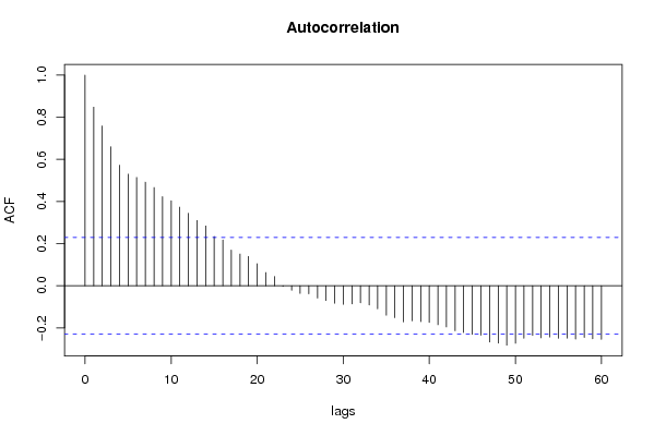
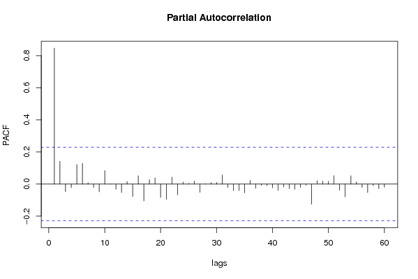
Title produced by software

(Partial) Autocorrelation Function

Date of computation

Thu, 04 Jun 2009 05:03:57 -0600

Cite this page as follows

Statistical Computations at FreeStatistics.org, Office for Research Development and Education, URL https://freestatistics.org/blog/index.php?v=date/2009/Jun/04/t1244113483sc95m5cqfbmt2uf.htm/, Retrieved Mon, 13 May 2024 23:06:58 +0000

Statistical Computations at FreeStatistics.org, Office for Research Development and Education, URL https://freestatistics.org/blog/index.php?pk=41593, Retrieved Mon, 13 May 2024 23:06:58 +0000

QR Codes:

Paste this QR Code to cite your computation.

Original text written by user:

IsPrivate?

No (this computation is public)

User-defined keywords

Estimated Impact

173

Family? (F = Feedback message, R = changed R code, M = changed R Module, P = changed Parameters, D = changed Data)

-     [Mean Plot] [Brutoschuld van d...] [2009-06-04 10:54:18] [ef653b42671acc8de32235b938c43afe]
- RMP     [(Partial) Autocorrelation Function] [Brutoschuld van d...] [2009-06-04 11:03:57] [2eea656d1ea82c4ced0e8e79cdac0617] [Current]
- RMPD      [Bootstrap Plot - Central Tendency] [Studio 100 maximu...] [2009-06-04 11:35:38] [ef653b42671acc8de32235b938c43afe] 
-   P         [Bootstrap Plot - Central Tendency] [Studio 100 maximu...] [2009-06-04 11:56:22] [ef653b42671acc8de32235b938c43afe] 
-   P           [Bootstrap Plot - Central Tendency] [Studio 100 maximu...] [2009-06-04 12:00:38] [ef653b42671acc8de32235b938c43afe] 
- RMPD          [Blocked Bootstrap Plot - Central Tendency] [Brutoschuld van d...] [2009-06-04 12:31:11] [ef653b42671acc8de32235b938c43afe] 
-   P             [Blocked Bootstrap Plot - Central Tendency] [Brutoschuld van d...] [2009-06-04 12:33:42] [ef653b42671acc8de32235b938c43afe] 
-   P               [Blocked Bootstrap Plot - Central Tendency] [Brutoschuld van d...] [2009-06-04 12:35:49] [ef653b42671acc8de32235b938c43afe] 
- RMPD              [Variability] [Studio 100 maximu...] [2009-06-04 13:04:21] [ef653b42671acc8de32235b938c43afe] 
- RMPD              [Standard Deviation Plot] [inschrijving nieu...] [2009-06-04 13:07:39] [ef653b42671acc8de32235b938c43afe] 
- RMPD              [Standard Deviation-Mean Plot] [inschrijving nieu...] [2009-06-04 13:14:37] [ef653b42671acc8de32235b938c43afe] 
-   P                 [Standard Deviation-Mean Plot] [inschrijving nieu...] [2009-06-07 11:50:31] [74be16979710d4c4e7c6647856088456] 
- RMP               [Variability] [Brutoschuld van d...] [2009-06-04 13:29:11] [ef653b42671acc8de32235b938c43afe] 
- RMP               [Standard Deviation Plot] [Brutoschuld van d...] [2009-06-04 13:30:21] [ef653b42671acc8de32235b938c43afe] 
- RMP               [Standard Deviation-Mean Plot] [Brutoschuld van d...] [2009-06-04 13:32:37] [ef653b42671acc8de32235b938c43afe] 
- RMPD              [Classical Decomposition] [inschrijving nieu...] [2009-06-04 13:58:57] [ef653b42671acc8de32235b938c43afe] 
-    D                [Classical Decomposition] [Brutoschuld van d...] [2009-06-04 14:13:36] [ef653b42671acc8de32235b938c43afe] 
- RM                  [Exponential Smoothing] [inschrijving nieu...] [2009-06-04 14:21:16] [ef653b42671acc8de32235b938c43afe] 
-   PD                  [Exponential Smoothing] [Bruto schuld van ...] [2009-06-07 16:49:36] [74be16979710d4c4e7c6647856088456] 

Feedback Forum

Post a new message

Dataseries X:

Download CSV

Histogram

Boxplots

Summary of computational transaction
Raw Input	view raw input (R code)
Raw Output	view raw output of R engine
Computing time	1 seconds
R Server	'George Udny Yule' @ 72.249.76.132

\begin{tabular}{lllllllll}
\hline
Summary of computational transaction \tabularnewline
Raw Input & view raw input (R code)  \tabularnewline
Raw Output & view raw output of R engine  \tabularnewline
Computing time & 1 seconds \tabularnewline
R Server & 'George Udny Yule' @ 72.249.76.132 \tabularnewline
\hline
\end{tabular}
%Source: https://freestatistics.org/blog/index.php?pk=41593&T=0

[TABLE]
[ROW][C]Summary of computational transaction[/C][/ROW]
[ROW][C]Raw Input[/C][C]view raw input (R code) [/C][/ROW]
[ROW][C]Raw Output[/C][C]view raw output of R engine [/C][/ROW]
[ROW][C]Computing time[/C][C]1 seconds[/C][/ROW]
[ROW][C]R Server[/C][C]'George Udny Yule' @ 72.249.76.132[/C][/ROW]
[/TABLE]
Source: https://freestatistics.org/blog/index.php?pk=41593&T=0

Globally Unique Identifier (entire table): ba.freestatistics.org/blog/index.php?pk=41593&T=0

As an alternative you can also use a QR Code:

The GUIDs for individual cells are displayed in the table below:

Summary of computational transaction
Raw Input	view raw input (R code)
Raw Output	view raw output of R engine
Computing time	1 seconds
R Server	'George Udny Yule' @ 72.249.76.132

Autocorrelation Function
Time lag k	ACF(k)	T-STAT	P-value
1	0.848027	7.2455	0
2	0.759002	6.4849	0
3	0.659751	5.6369	0
4	0.572154	4.8885	3e-06
5	0.529723	4.526	1.1e-05
6	0.513947	4.3912	1.9e-05
7	0.491801	4.202	3.7e-05
8	0.466063	3.982	8e-05
9	0.423067	3.6147	0.000275
10	0.403452	3.4471	0.000472
11	0.373239	3.189	0.001052
12	0.344044	2.9395	0.0022
13	0.309928	2.648	0.004958
14	0.283712	2.424	0.008913
15	0.233986	1.9992	0.024656
16	0.217013	1.8542	0.033878
17	0.169132	1.4451	0.07636
18	0.150543	1.2862	0.101212
19	0.138922	1.187	0.119547
20	0.104299	0.8911	0.187893
21	0.062567	0.5346	0.297284
22	0.043799	0.3742	0.354662
23	-0.003854	-0.0329	0.486911
24	-0.021445	-0.1832	0.427564
25	-0.036485	-0.3117	0.378068
26	-0.038366	-0.3278	0.372
27	-0.058266	-0.4978	0.310051
28	-0.0705	-0.6024	0.274403
29	-0.08331	-0.7118	0.239429
30	-0.088642	-0.7574	0.225638
31	-0.08611	-0.7357	0.232127
32	-0.081235	-0.6941	0.244921
33	-0.091833	-0.7846	0.217608
34	-0.109527	-0.9358	0.176231
35	-0.140298	-1.1987	0.11726
36	-0.151945	-1.2982	0.09915
37	-0.171697	-1.467	0.073338
38	-0.166721	-1.4245	0.079287
39	-0.170483	-1.4566	0.074757
40	-0.174152	-1.488	0.070535
41	-0.185509	-1.585	0.058645
42	-0.195749	-1.6725	0.049356
43	-0.213609	-1.8251	0.03604
44	-0.222024	-1.897	0.030894
45	-0.231604	-1.9788	0.025804
46	-0.235125	-2.0089	0.024123
47	-0.267535	-2.2858	0.012585
48	-0.272933	-2.3319	0.011233
49	-0.282234	-2.4114	0.009204
50	-0.273498	-2.3368	0.011099
51	-0.24972	-2.1336	0.018118
52	-0.236046	-2.0168	0.023699
53	-0.247243	-2.1124	0.019035
54	-0.243342	-2.0791	0.02056
55	-0.24971	-2.1335	0.018121
56	-0.248553	-2.1236	0.018545
57	-0.253155	-2.163	0.01691
58	-0.245459	-2.0972	0.01972
59	-0.251751	-2.151	0.017395
60	-0.254647	-2.1757	0.016408

\begin{tabular}{lllllllll}
\hline
Autocorrelation Function \tabularnewline
Time lag k & ACF(k) & T-STAT & P-value \tabularnewline
1 & 0.848027 & 7.2455 & 0 \tabularnewline
2 & 0.759002 & 6.4849 & 0 \tabularnewline
3 & 0.659751 & 5.6369 & 0 \tabularnewline
4 & 0.572154 & 4.8885 & 3e-06 \tabularnewline
5 & 0.529723 & 4.526 & 1.1e-05 \tabularnewline
6 & 0.513947 & 4.3912 & 1.9e-05 \tabularnewline
7 & 0.491801 & 4.202 & 3.7e-05 \tabularnewline
8 & 0.466063 & 3.982 & 8e-05 \tabularnewline
9 & 0.423067 & 3.6147 & 0.000275 \tabularnewline
10 & 0.403452 & 3.4471 & 0.000472 \tabularnewline
11 & 0.373239 & 3.189 & 0.001052 \tabularnewline
12 & 0.344044 & 2.9395 & 0.0022 \tabularnewline
13 & 0.309928 & 2.648 & 0.004958 \tabularnewline
14 & 0.283712 & 2.424 & 0.008913 \tabularnewline
15 & 0.233986 & 1.9992 & 0.024656 \tabularnewline
16 & 0.217013 & 1.8542 & 0.033878 \tabularnewline
17 & 0.169132 & 1.4451 & 0.07636 \tabularnewline
18 & 0.150543 & 1.2862 & 0.101212 \tabularnewline
19 & 0.138922 & 1.187 & 0.119547 \tabularnewline
20 & 0.104299 & 0.8911 & 0.187893 \tabularnewline
21 & 0.062567 & 0.5346 & 0.297284 \tabularnewline
22 & 0.043799 & 0.3742 & 0.354662 \tabularnewline
23 & -0.003854 & -0.0329 & 0.486911 \tabularnewline
24 & -0.021445 & -0.1832 & 0.427564 \tabularnewline
25 & -0.036485 & -0.3117 & 0.378068 \tabularnewline
26 & -0.038366 & -0.3278 & 0.372 \tabularnewline
27 & -0.058266 & -0.4978 & 0.310051 \tabularnewline
28 & -0.0705 & -0.6024 & 0.274403 \tabularnewline
29 & -0.08331 & -0.7118 & 0.239429 \tabularnewline
30 & -0.088642 & -0.7574 & 0.225638 \tabularnewline
31 & -0.08611 & -0.7357 & 0.232127 \tabularnewline
32 & -0.081235 & -0.6941 & 0.244921 \tabularnewline
33 & -0.091833 & -0.7846 & 0.217608 \tabularnewline
34 & -0.109527 & -0.9358 & 0.176231 \tabularnewline
35 & -0.140298 & -1.1987 & 0.11726 \tabularnewline
36 & -0.151945 & -1.2982 & 0.09915 \tabularnewline
37 & -0.171697 & -1.467 & 0.073338 \tabularnewline
38 & -0.166721 & -1.4245 & 0.079287 \tabularnewline
39 & -0.170483 & -1.4566 & 0.074757 \tabularnewline
40 & -0.174152 & -1.488 & 0.070535 \tabularnewline
41 & -0.185509 & -1.585 & 0.058645 \tabularnewline
42 & -0.195749 & -1.6725 & 0.049356 \tabularnewline
43 & -0.213609 & -1.8251 & 0.03604 \tabularnewline
44 & -0.222024 & -1.897 & 0.030894 \tabularnewline
45 & -0.231604 & -1.9788 & 0.025804 \tabularnewline
46 & -0.235125 & -2.0089 & 0.024123 \tabularnewline
47 & -0.267535 & -2.2858 & 0.012585 \tabularnewline
48 & -0.272933 & -2.3319 & 0.011233 \tabularnewline
49 & -0.282234 & -2.4114 & 0.009204 \tabularnewline
50 & -0.273498 & -2.3368 & 0.011099 \tabularnewline
51 & -0.24972 & -2.1336 & 0.018118 \tabularnewline
52 & -0.236046 & -2.0168 & 0.023699 \tabularnewline
53 & -0.247243 & -2.1124 & 0.019035 \tabularnewline
54 & -0.243342 & -2.0791 & 0.02056 \tabularnewline
55 & -0.24971 & -2.1335 & 0.018121 \tabularnewline
56 & -0.248553 & -2.1236 & 0.018545 \tabularnewline
57 & -0.253155 & -2.163 & 0.01691 \tabularnewline
58 & -0.245459 & -2.0972 & 0.01972 \tabularnewline
59 & -0.251751 & -2.151 & 0.017395 \tabularnewline
60 & -0.254647 & -2.1757 & 0.016408 \tabularnewline
\hline
\end{tabular}
%Source: https://freestatistics.org/blog/index.php?pk=41593&T=1

[TABLE]
[ROW][C]Autocorrelation Function[/C][/ROW]
[ROW][C]Time lag k[/C][C]ACF(k)[/C][C]T-STAT[/C][C]P-value[/C][/ROW]
[ROW][C]1[/C][C]0.848027[/C][C]7.2455[/C][C]0[/C][/ROW]
[ROW][C]2[/C][C]0.759002[/C][C]6.4849[/C][C]0[/C][/ROW]
[ROW][C]3[/C][C]0.659751[/C][C]5.6369[/C][C]0[/C][/ROW]
[ROW][C]4[/C][C]0.572154[/C][C]4.8885[/C][C]3e-06[/C][/ROW]
[ROW][C]5[/C][C]0.529723[/C][C]4.526[/C][C]1.1e-05[/C][/ROW]
[ROW][C]6[/C][C]0.513947[/C][C]4.3912[/C][C]1.9e-05[/C][/ROW]
[ROW][C]7[/C][C]0.491801[/C][C]4.202[/C][C]3.7e-05[/C][/ROW]
[ROW][C]8[/C][C]0.466063[/C][C]3.982[/C][C]8e-05[/C][/ROW]
[ROW][C]9[/C][C]0.423067[/C][C]3.6147[/C][C]0.000275[/C][/ROW]
[ROW][C]10[/C][C]0.403452[/C][C]3.4471[/C][C]0.000472[/C][/ROW]
[ROW][C]11[/C][C]0.373239[/C][C]3.189[/C][C]0.001052[/C][/ROW]
[ROW][C]12[/C][C]0.344044[/C][C]2.9395[/C][C]0.0022[/C][/ROW]
[ROW][C]13[/C][C]0.309928[/C][C]2.648[/C][C]0.004958[/C][/ROW]
[ROW][C]14[/C][C]0.283712[/C][C]2.424[/C][C]0.008913[/C][/ROW]
[ROW][C]15[/C][C]0.233986[/C][C]1.9992[/C][C]0.024656[/C][/ROW]
[ROW][C]16[/C][C]0.217013[/C][C]1.8542[/C][C]0.033878[/C][/ROW]
[ROW][C]17[/C][C]0.169132[/C][C]1.4451[/C][C]0.07636[/C][/ROW]
[ROW][C]18[/C][C]0.150543[/C][C]1.2862[/C][C]0.101212[/C][/ROW]
[ROW][C]19[/C][C]0.138922[/C][C]1.187[/C][C]0.119547[/C][/ROW]
[ROW][C]20[/C][C]0.104299[/C][C]0.8911[/C][C]0.187893[/C][/ROW]
[ROW][C]21[/C][C]0.062567[/C][C]0.5346[/C][C]0.297284[/C][/ROW]
[ROW][C]22[/C][C]0.043799[/C][C]0.3742[/C][C]0.354662[/C][/ROW]
[ROW][C]23[/C][C]-0.003854[/C][C]-0.0329[/C][C]0.486911[/C][/ROW]
[ROW][C]24[/C][C]-0.021445[/C][C]-0.1832[/C][C]0.427564[/C][/ROW]
[ROW][C]25[/C][C]-0.036485[/C][C]-0.3117[/C][C]0.378068[/C][/ROW]
[ROW][C]26[/C][C]-0.038366[/C][C]-0.3278[/C][C]0.372[/C][/ROW]
[ROW][C]27[/C][C]-0.058266[/C][C]-0.4978[/C][C]0.310051[/C][/ROW]
[ROW][C]28[/C][C]-0.0705[/C][C]-0.6024[/C][C]0.274403[/C][/ROW]
[ROW][C]29[/C][C]-0.08331[/C][C]-0.7118[/C][C]0.239429[/C][/ROW]
[ROW][C]30[/C][C]-0.088642[/C][C]-0.7574[/C][C]0.225638[/C][/ROW]
[ROW][C]31[/C][C]-0.08611[/C][C]-0.7357[/C][C]0.232127[/C][/ROW]
[ROW][C]32[/C][C]-0.081235[/C][C]-0.6941[/C][C]0.244921[/C][/ROW]
[ROW][C]33[/C][C]-0.091833[/C][C]-0.7846[/C][C]0.217608[/C][/ROW]
[ROW][C]34[/C][C]-0.109527[/C][C]-0.9358[/C][C]0.176231[/C][/ROW]
[ROW][C]35[/C][C]-0.140298[/C][C]-1.1987[/C][C]0.11726[/C][/ROW]
[ROW][C]36[/C][C]-0.151945[/C][C]-1.2982[/C][C]0.09915[/C][/ROW]
[ROW][C]37[/C][C]-0.171697[/C][C]-1.467[/C][C]0.073338[/C][/ROW]
[ROW][C]38[/C][C]-0.166721[/C][C]-1.4245[/C][C]0.079287[/C][/ROW]
[ROW][C]39[/C][C]-0.170483[/C][C]-1.4566[/C][C]0.074757[/C][/ROW]
[ROW][C]40[/C][C]-0.174152[/C][C]-1.488[/C][C]0.070535[/C][/ROW]
[ROW][C]41[/C][C]-0.185509[/C][C]-1.585[/C][C]0.058645[/C][/ROW]
[ROW][C]42[/C][C]-0.195749[/C][C]-1.6725[/C][C]0.049356[/C][/ROW]
[ROW][C]43[/C][C]-0.213609[/C][C]-1.8251[/C][C]0.03604[/C][/ROW]
[ROW][C]44[/C][C]-0.222024[/C][C]-1.897[/C][C]0.030894[/C][/ROW]
[ROW][C]45[/C][C]-0.231604[/C][C]-1.9788[/C][C]0.025804[/C][/ROW]
[ROW][C]46[/C][C]-0.235125[/C][C]-2.0089[/C][C]0.024123[/C][/ROW]
[ROW][C]47[/C][C]-0.267535[/C][C]-2.2858[/C][C]0.012585[/C][/ROW]
[ROW][C]48[/C][C]-0.272933[/C][C]-2.3319[/C][C]0.011233[/C][/ROW]
[ROW][C]49[/C][C]-0.282234[/C][C]-2.4114[/C][C]0.009204[/C][/ROW]
[ROW][C]50[/C][C]-0.273498[/C][C]-2.3368[/C][C]0.011099[/C][/ROW]
[ROW][C]51[/C][C]-0.24972[/C][C]-2.1336[/C][C]0.018118[/C][/ROW]
[ROW][C]52[/C][C]-0.236046[/C][C]-2.0168[/C][C]0.023699[/C][/ROW]
[ROW][C]53[/C][C]-0.247243[/C][C]-2.1124[/C][C]0.019035[/C][/ROW]
[ROW][C]54[/C][C]-0.243342[/C][C]-2.0791[/C][C]0.02056[/C][/ROW]
[ROW][C]55[/C][C]-0.24971[/C][C]-2.1335[/C][C]0.018121[/C][/ROW]
[ROW][C]56[/C][C]-0.248553[/C][C]-2.1236[/C][C]0.018545[/C][/ROW]
[ROW][C]57[/C][C]-0.253155[/C][C]-2.163[/C][C]0.01691[/C][/ROW]
[ROW][C]58[/C][C]-0.245459[/C][C]-2.0972[/C][C]0.01972[/C][/ROW]
[ROW][C]59[/C][C]-0.251751[/C][C]-2.151[/C][C]0.017395[/C][/ROW]
[ROW][C]60[/C][C]-0.254647[/C][C]-2.1757[/C][C]0.016408[/C][/ROW]
[/TABLE]
Source: https://freestatistics.org/blog/index.php?pk=41593&T=1

Globally Unique Identifier (entire table): ba.freestatistics.org/blog/index.php?pk=41593&T=1

As an alternative you can also use a QR Code:

The GUIDs for individual cells are displayed in the table below:

Autocorrelation Function
Time lag k	ACF(k)	T-STAT	P-value
1	0.848027	7.2455	0
2	0.759002	6.4849	0
3	0.659751	5.6369	0
4	0.572154	4.8885	3e-06
5	0.529723	4.526	1.1e-05
6	0.513947	4.3912	1.9e-05
7	0.491801	4.202	3.7e-05
8	0.466063	3.982	8e-05
9	0.423067	3.6147	0.000275
10	0.403452	3.4471	0.000472
11	0.373239	3.189	0.001052
12	0.344044	2.9395	0.0022
13	0.309928	2.648	0.004958
14	0.283712	2.424	0.008913
15	0.233986	1.9992	0.024656
16	0.217013	1.8542	0.033878
17	0.169132	1.4451	0.07636
18	0.150543	1.2862	0.101212
19	0.138922	1.187	0.119547
20	0.104299	0.8911	0.187893
21	0.062567	0.5346	0.297284
22	0.043799	0.3742	0.354662
23	-0.003854	-0.0329	0.486911
24	-0.021445	-0.1832	0.427564
25	-0.036485	-0.3117	0.378068
26	-0.038366	-0.3278	0.372
27	-0.058266	-0.4978	0.310051
28	-0.0705	-0.6024	0.274403
29	-0.08331	-0.7118	0.239429
30	-0.088642	-0.7574	0.225638
31	-0.08611	-0.7357	0.232127
32	-0.081235	-0.6941	0.244921
33	-0.091833	-0.7846	0.217608
34	-0.109527	-0.9358	0.176231
35	-0.140298	-1.1987	0.11726
36	-0.151945	-1.2982	0.09915
37	-0.171697	-1.467	0.073338
38	-0.166721	-1.4245	0.079287
39	-0.170483	-1.4566	0.074757
40	-0.174152	-1.488	0.070535
41	-0.185509	-1.585	0.058645
42	-0.195749	-1.6725	0.049356
43	-0.213609	-1.8251	0.03604
44	-0.222024	-1.897	0.030894
45	-0.231604	-1.9788	0.025804
46	-0.235125	-2.0089	0.024123
47	-0.267535	-2.2858	0.012585
48	-0.272933	-2.3319	0.011233
49	-0.282234	-2.4114	0.009204
50	-0.273498	-2.3368	0.011099
51	-0.24972	-2.1336	0.018118
52	-0.236046	-2.0168	0.023699
53	-0.247243	-2.1124	0.019035
54	-0.243342	-2.0791	0.02056
55	-0.24971	-2.1335	0.018121
56	-0.248553	-2.1236	0.018545
57	-0.253155	-2.163	0.01691
58	-0.245459	-2.0972	0.01972
59	-0.251751	-2.151	0.017395
60	-0.254647	-2.1757	0.016408

Partial Autocorrelation Function
Time lag k	PACF(k)	T-STAT	P-value
1	0.848027	7.2455	0
2	0.141901	1.2124	0.114634
3	-0.046891	-0.4006	0.344928
4	-0.02246	-0.1919	0.424179
5	0.122229	1.0443	0.14989
6	0.129245	1.1043	0.136552
7	0.008286	0.0708	0.471877
8	-0.021374	-0.1826	0.427802
9	-0.048712	-0.4162	0.339245
10	0.084238	0.7197	0.236994
11	0.001096	0.0094	0.496276
12	-0.032139	-0.2746	0.3922
13	-0.052417	-0.4478	0.327794
14	0.015606	0.1333	0.447146
15	-0.077089	-0.6586	0.256098
16	0.051411	0.4393	0.330886
17	-0.10486	-0.8959	0.186618
18	0.027447	0.2345	0.407625
19	0.039153	0.3345	0.369472
20	-0.083343	-0.7121	0.239342
21	-0.095215	-0.8135	0.209284
22	0.043574	0.3723	0.355375
23	-0.067284	-0.5749	0.283572
24	0.012883	0.1101	0.456326
25	0.004212	0.036	0.485696
26	0.018993	0.1623	0.435767
27	-0.051653	-0.4413	0.33014
28	0.002263	0.0193	0.492313
29	0.009711	0.083	0.467049
30	0.010533	0.09	0.464268
31	0.057105	0.4879	0.31354
32	-0.021147	-0.1807	0.428559
33	-0.040602	-0.3469	0.364831
34	-0.040853	-0.3491	0.364028
35	-0.054448	-0.4652	0.321586
36	0.023988	0.205	0.419089
37	-0.026885	-0.2297	0.409482
38	-0.007741	-0.0661	0.473725
39	-0.009741	-0.0832	0.466948
40	-0.023297	-0.199	0.421389
41	-0.039	-0.3332	0.369962
42	-0.017683	-0.1511	0.440162
43	-0.029097	-0.2486	0.402182
44	-0.032752	-0.2798	0.390198
45	-0.020598	-0.176	0.430395
46	-0.00699	-0.0597	0.476269
47	-0.125975	-1.0763	0.142663
48	0.021592	0.1845	0.427072
49	0.01778	0.1519	0.439838
50	0.017518	0.1497	0.440718
51	0.052506	0.4486	0.327521
52	-0.038447	-0.3285	0.371739
53	-0.079236	-0.677	0.250276
54	0.052119	0.4453	0.328707
55	0.013896	0.1187	0.452909
56	-0.020639	-0.1763	0.430257
57	-0.053018	-0.453	0.325951
58	-0.01004	-0.0858	0.465936
59	-0.028164	-0.2406	0.405257
60	-0.019859	-0.1697	0.432867

\begin{tabular}{lllllllll}
\hline
Partial Autocorrelation Function \tabularnewline
Time lag k & PACF(k) & T-STAT & P-value \tabularnewline
1 & 0.848027 & 7.2455 & 0 \tabularnewline
2 & 0.141901 & 1.2124 & 0.114634 \tabularnewline
3 & -0.046891 & -0.4006 & 0.344928 \tabularnewline
4 & -0.02246 & -0.1919 & 0.424179 \tabularnewline
5 & 0.122229 & 1.0443 & 0.14989 \tabularnewline
6 & 0.129245 & 1.1043 & 0.136552 \tabularnewline
7 & 0.008286 & 0.0708 & 0.471877 \tabularnewline
8 & -0.021374 & -0.1826 & 0.427802 \tabularnewline
9 & -0.048712 & -0.4162 & 0.339245 \tabularnewline
10 & 0.084238 & 0.7197 & 0.236994 \tabularnewline
11 & 0.001096 & 0.0094 & 0.496276 \tabularnewline
12 & -0.032139 & -0.2746 & 0.3922 \tabularnewline
13 & -0.052417 & -0.4478 & 0.327794 \tabularnewline
14 & 0.015606 & 0.1333 & 0.447146 \tabularnewline
15 & -0.077089 & -0.6586 & 0.256098 \tabularnewline
16 & 0.051411 & 0.4393 & 0.330886 \tabularnewline
17 & -0.10486 & -0.8959 & 0.186618 \tabularnewline
18 & 0.027447 & 0.2345 & 0.407625 \tabularnewline
19 & 0.039153 & 0.3345 & 0.369472 \tabularnewline
20 & -0.083343 & -0.7121 & 0.239342 \tabularnewline
21 & -0.095215 & -0.8135 & 0.209284 \tabularnewline
22 & 0.043574 & 0.3723 & 0.355375 \tabularnewline
23 & -0.067284 & -0.5749 & 0.283572 \tabularnewline
24 & 0.012883 & 0.1101 & 0.456326 \tabularnewline
25 & 0.004212 & 0.036 & 0.485696 \tabularnewline
26 & 0.018993 & 0.1623 & 0.435767 \tabularnewline
27 & -0.051653 & -0.4413 & 0.33014 \tabularnewline
28 & 0.002263 & 0.0193 & 0.492313 \tabularnewline
29 & 0.009711 & 0.083 & 0.467049 \tabularnewline
30 & 0.010533 & 0.09 & 0.464268 \tabularnewline
31 & 0.057105 & 0.4879 & 0.31354 \tabularnewline
32 & -0.021147 & -0.1807 & 0.428559 \tabularnewline
33 & -0.040602 & -0.3469 & 0.364831 \tabularnewline
34 & -0.040853 & -0.3491 & 0.364028 \tabularnewline
35 & -0.054448 & -0.4652 & 0.321586 \tabularnewline
36 & 0.023988 & 0.205 & 0.419089 \tabularnewline
37 & -0.026885 & -0.2297 & 0.409482 \tabularnewline
38 & -0.007741 & -0.0661 & 0.473725 \tabularnewline
39 & -0.009741 & -0.0832 & 0.466948 \tabularnewline
40 & -0.023297 & -0.199 & 0.421389 \tabularnewline
41 & -0.039 & -0.3332 & 0.369962 \tabularnewline
42 & -0.017683 & -0.1511 & 0.440162 \tabularnewline
43 & -0.029097 & -0.2486 & 0.402182 \tabularnewline
44 & -0.032752 & -0.2798 & 0.390198 \tabularnewline
45 & -0.020598 & -0.176 & 0.430395 \tabularnewline
46 & -0.00699 & -0.0597 & 0.476269 \tabularnewline
47 & -0.125975 & -1.0763 & 0.142663 \tabularnewline
48 & 0.021592 & 0.1845 & 0.427072 \tabularnewline
49 & 0.01778 & 0.1519 & 0.439838 \tabularnewline
50 & 0.017518 & 0.1497 & 0.440718 \tabularnewline
51 & 0.052506 & 0.4486 & 0.327521 \tabularnewline
52 & -0.038447 & -0.3285 & 0.371739 \tabularnewline
53 & -0.079236 & -0.677 & 0.250276 \tabularnewline
54 & 0.052119 & 0.4453 & 0.328707 \tabularnewline
55 & 0.013896 & 0.1187 & 0.452909 \tabularnewline
56 & -0.020639 & -0.1763 & 0.430257 \tabularnewline
57 & -0.053018 & -0.453 & 0.325951 \tabularnewline
58 & -0.01004 & -0.0858 & 0.465936 \tabularnewline
59 & -0.028164 & -0.2406 & 0.405257 \tabularnewline
60 & -0.019859 & -0.1697 & 0.432867 \tabularnewline
\hline
\end{tabular}
%Source: https://freestatistics.org/blog/index.php?pk=41593&T=2

[TABLE]
[ROW][C]Partial Autocorrelation Function[/C][/ROW]
[ROW][C]Time lag k[/C][C]PACF(k)[/C][C]T-STAT[/C][C]P-value[/C][/ROW]
[ROW][C]1[/C][C]0.848027[/C][C]7.2455[/C][C]0[/C][/ROW]
[ROW][C]2[/C][C]0.141901[/C][C]1.2124[/C][C]0.114634[/C][/ROW]
[ROW][C]3[/C][C]-0.046891[/C][C]-0.4006[/C][C]0.344928[/C][/ROW]
[ROW][C]4[/C][C]-0.02246[/C][C]-0.1919[/C][C]0.424179[/C][/ROW]
[ROW][C]5[/C][C]0.122229[/C][C]1.0443[/C][C]0.14989[/C][/ROW]
[ROW][C]6[/C][C]0.129245[/C][C]1.1043[/C][C]0.136552[/C][/ROW]
[ROW][C]7[/C][C]0.008286[/C][C]0.0708[/C][C]0.471877[/C][/ROW]
[ROW][C]8[/C][C]-0.021374[/C][C]-0.1826[/C][C]0.427802[/C][/ROW]
[ROW][C]9[/C][C]-0.048712[/C][C]-0.4162[/C][C]0.339245[/C][/ROW]
[ROW][C]10[/C][C]0.084238[/C][C]0.7197[/C][C]0.236994[/C][/ROW]
[ROW][C]11[/C][C]0.001096[/C][C]0.0094[/C][C]0.496276[/C][/ROW]
[ROW][C]12[/C][C]-0.032139[/C][C]-0.2746[/C][C]0.3922[/C][/ROW]
[ROW][C]13[/C][C]-0.052417[/C][C]-0.4478[/C][C]0.327794[/C][/ROW]
[ROW][C]14[/C][C]0.015606[/C][C]0.1333[/C][C]0.447146[/C][/ROW]
[ROW][C]15[/C][C]-0.077089[/C][C]-0.6586[/C][C]0.256098[/C][/ROW]
[ROW][C]16[/C][C]0.051411[/C][C]0.4393[/C][C]0.330886[/C][/ROW]
[ROW][C]17[/C][C]-0.10486[/C][C]-0.8959[/C][C]0.186618[/C][/ROW]
[ROW][C]18[/C][C]0.027447[/C][C]0.2345[/C][C]0.407625[/C][/ROW]
[ROW][C]19[/C][C]0.039153[/C][C]0.3345[/C][C]0.369472[/C][/ROW]
[ROW][C]20[/C][C]-0.083343[/C][C]-0.7121[/C][C]0.239342[/C][/ROW]
[ROW][C]21[/C][C]-0.095215[/C][C]-0.8135[/C][C]0.209284[/C][/ROW]
[ROW][C]22[/C][C]0.043574[/C][C]0.3723[/C][C]0.355375[/C][/ROW]
[ROW][C]23[/C][C]-0.067284[/C][C]-0.5749[/C][C]0.283572[/C][/ROW]
[ROW][C]24[/C][C]0.012883[/C][C]0.1101[/C][C]0.456326[/C][/ROW]
[ROW][C]25[/C][C]0.004212[/C][C]0.036[/C][C]0.485696[/C][/ROW]
[ROW][C]26[/C][C]0.018993[/C][C]0.1623[/C][C]0.435767[/C][/ROW]
[ROW][C]27[/C][C]-0.051653[/C][C]-0.4413[/C][C]0.33014[/C][/ROW]
[ROW][C]28[/C][C]0.002263[/C][C]0.0193[/C][C]0.492313[/C][/ROW]
[ROW][C]29[/C][C]0.009711[/C][C]0.083[/C][C]0.467049[/C][/ROW]
[ROW][C]30[/C][C]0.010533[/C][C]0.09[/C][C]0.464268[/C][/ROW]
[ROW][C]31[/C][C]0.057105[/C][C]0.4879[/C][C]0.31354[/C][/ROW]
[ROW][C]32[/C][C]-0.021147[/C][C]-0.1807[/C][C]0.428559[/C][/ROW]
[ROW][C]33[/C][C]-0.040602[/C][C]-0.3469[/C][C]0.364831[/C][/ROW]
[ROW][C]34[/C][C]-0.040853[/C][C]-0.3491[/C][C]0.364028[/C][/ROW]
[ROW][C]35[/C][C]-0.054448[/C][C]-0.4652[/C][C]0.321586[/C][/ROW]
[ROW][C]36[/C][C]0.023988[/C][C]0.205[/C][C]0.419089[/C][/ROW]
[ROW][C]37[/C][C]-0.026885[/C][C]-0.2297[/C][C]0.409482[/C][/ROW]
[ROW][C]38[/C][C]-0.007741[/C][C]-0.0661[/C][C]0.473725[/C][/ROW]
[ROW][C]39[/C][C]-0.009741[/C][C]-0.0832[/C][C]0.466948[/C][/ROW]
[ROW][C]40[/C][C]-0.023297[/C][C]-0.199[/C][C]0.421389[/C][/ROW]
[ROW][C]41[/C][C]-0.039[/C][C]-0.3332[/C][C]0.369962[/C][/ROW]
[ROW][C]42[/C][C]-0.017683[/C][C]-0.1511[/C][C]0.440162[/C][/ROW]
[ROW][C]43[/C][C]-0.029097[/C][C]-0.2486[/C][C]0.402182[/C][/ROW]
[ROW][C]44[/C][C]-0.032752[/C][C]-0.2798[/C][C]0.390198[/C][/ROW]
[ROW][C]45[/C][C]-0.020598[/C][C]-0.176[/C][C]0.430395[/C][/ROW]
[ROW][C]46[/C][C]-0.00699[/C][C]-0.0597[/C][C]0.476269[/C][/ROW]
[ROW][C]47[/C][C]-0.125975[/C][C]-1.0763[/C][C]0.142663[/C][/ROW]
[ROW][C]48[/C][C]0.021592[/C][C]0.1845[/C][C]0.427072[/C][/ROW]
[ROW][C]49[/C][C]0.01778[/C][C]0.1519[/C][C]0.439838[/C][/ROW]
[ROW][C]50[/C][C]0.017518[/C][C]0.1497[/C][C]0.440718[/C][/ROW]
[ROW][C]51[/C][C]0.052506[/C][C]0.4486[/C][C]0.327521[/C][/ROW]
[ROW][C]52[/C][C]-0.038447[/C][C]-0.3285[/C][C]0.371739[/C][/ROW]
[ROW][C]53[/C][C]-0.079236[/C][C]-0.677[/C][C]0.250276[/C][/ROW]
[ROW][C]54[/C][C]0.052119[/C][C]0.4453[/C][C]0.328707[/C][/ROW]
[ROW][C]55[/C][C]0.013896[/C][C]0.1187[/C][C]0.452909[/C][/ROW]
[ROW][C]56[/C][C]-0.020639[/C][C]-0.1763[/C][C]0.430257[/C][/ROW]
[ROW][C]57[/C][C]-0.053018[/C][C]-0.453[/C][C]0.325951[/C][/ROW]
[ROW][C]58[/C][C]-0.01004[/C][C]-0.0858[/C][C]0.465936[/C][/ROW]
[ROW][C]59[/C][C]-0.028164[/C][C]-0.2406[/C][C]0.405257[/C][/ROW]
[ROW][C]60[/C][C]-0.019859[/C][C]-0.1697[/C][C]0.432867[/C][/ROW]
[/TABLE]
Source: https://freestatistics.org/blog/index.php?pk=41593&T=2

Globally Unique Identifier (entire table): ba.freestatistics.org/blog/index.php?pk=41593&T=2

As an alternative you can also use a QR Code:

The GUIDs for individual cells are displayed in the table below:

Partial Autocorrelation Function
Time lag k	PACF(k)	T-STAT	P-value
1	0.848027	7.2455	0
2	0.141901	1.2124	0.114634
3	-0.046891	-0.4006	0.344928
4	-0.02246	-0.1919	0.424179
5	0.122229	1.0443	0.14989
6	0.129245	1.1043	0.136552
7	0.008286	0.0708	0.471877
8	-0.021374	-0.1826	0.427802
9	-0.048712	-0.4162	0.339245
10	0.084238	0.7197	0.236994
11	0.001096	0.0094	0.496276
12	-0.032139	-0.2746	0.3922
13	-0.052417	-0.4478	0.327794
14	0.015606	0.1333	0.447146
15	-0.077089	-0.6586	0.256098
16	0.051411	0.4393	0.330886
17	-0.10486	-0.8959	0.186618
18	0.027447	0.2345	0.407625
19	0.039153	0.3345	0.369472
20	-0.083343	-0.7121	0.239342
21	-0.095215	-0.8135	0.209284
22	0.043574	0.3723	0.355375
23	-0.067284	-0.5749	0.283572
24	0.012883	0.1101	0.456326
25	0.004212	0.036	0.485696
26	0.018993	0.1623	0.435767
27	-0.051653	-0.4413	0.33014
28	0.002263	0.0193	0.492313
29	0.009711	0.083	0.467049
30	0.010533	0.09	0.464268
31	0.057105	0.4879	0.31354
32	-0.021147	-0.1807	0.428559
33	-0.040602	-0.3469	0.364831
34	-0.040853	-0.3491	0.364028
35	-0.054448	-0.4652	0.321586
36	0.023988	0.205	0.419089
37	-0.026885	-0.2297	0.409482
38	-0.007741	-0.0661	0.473725
39	-0.009741	-0.0832	0.466948
40	-0.023297	-0.199	0.421389
41	-0.039	-0.3332	0.369962
42	-0.017683	-0.1511	0.440162
43	-0.029097	-0.2486	0.402182
44	-0.032752	-0.2798	0.390198
45	-0.020598	-0.176	0.430395
46	-0.00699	-0.0597	0.476269
47	-0.125975	-1.0763	0.142663
48	0.021592	0.1845	0.427072
49	0.01778	0.1519	0.439838
50	0.017518	0.1497	0.440718
51	0.052506	0.4486	0.327521
52	-0.038447	-0.3285	0.371739
53	-0.079236	-0.677	0.250276
54	0.052119	0.4453	0.328707
55	0.013896	0.1187	0.452909
56	-0.020639	-0.1763	0.430257
57	-0.053018	-0.453	0.325951
58	-0.01004	-0.0858	0.465936
59	-0.028164	-0.2406	0.405257
60	-0.019859	-0.1697	0.432867

Figure 1

PNG link

Postscript link

PDF link

Figure 2

PNG link

Postscript link

PDF link

Parameters (Session):

par1 = 60 ; par2 = 1 ; par3 = 0 ; par4 = 0 ; par5 = 12 ;

Parameters (R input):

par1 = 60 ; par2 = 1 ; par3 = 0 ; par4 = 0 ; par5 = 12 ;

R code (references can be found in the software module):

if (par1 == 'Default') {
par1 = 10*log10(length(x))
} else {
par1 <- as.numeric(par1)
}
par2 <- as.numeric(par2)
par3 <- as.numeric(par3)
par4 <- as.numeric(par4)
par5 <- as.numeric(par5)
if (par2 == 0) {
x <- log(x)
} else {
x <- (x ^ par2 - 1) / par2
}
if (par3 > 0) x <- diff(x,lag=1,difference=par3)
if (par4 > 0) x <- diff(x,lag=par5,difference=par4)
bitmap(file='pic1.png')
racf <- acf(x,par1,main='Autocorrelation',xlab='lags',ylab='ACF')
dev.off()
bitmap(file='pic2.png')
rpacf <- pacf(x,par1,main='Partial Autocorrelation',xlab='lags',ylab='PACF')
dev.off()
(myacf <- c(racf$acf))
(mypacf <- c(rpacf$acf))
lengthx <- length(x)
sqrtn <- sqrt(lengthx)
load(file='createtable')
a<-table.start()
a<-table.row.start(a)
a<-table.element(a,'Autocorrelation Function',4,TRUE)
a<-table.row.end(a)
a<-table.row.start(a)
a<-table.element(a,'Time lag k',header=TRUE)
a<-table.element(a,hyperlink('basics.htm','ACF(k)','click here for more information about the Autocorrelation Function'),header=TRUE)
a<-table.element(a,'T-STAT',header=TRUE)
a<-table.element(a,'P-value',header=TRUE)
a<-table.row.end(a)
for (i in 2:(par1+1)) {
a<-table.row.start(a)
a<-table.element(a,i-1,header=TRUE)
a<-table.element(a,round(myacf[i],6))
mytstat <- myacf[i]*sqrtn
a<-table.element(a,round(mytstat,4))
a<-table.element(a,round(1-pt(abs(mytstat),lengthx),6))
a<-table.row.end(a)
}
a<-table.end(a)
table.save(a,file='mytable.tab')
a<-table.start()
a<-table.row.start(a)
a<-table.element(a,'Partial Autocorrelation Function',4,TRUE)
a<-table.row.end(a)
a<-table.row.start(a)
a<-table.element(a,'Time lag k',header=TRUE)
a<-table.element(a,hyperlink('basics.htm','PACF(k)','click here for more information about the Partial Autocorrelation Function'),header=TRUE)
a<-table.element(a,'T-STAT',header=TRUE)
a<-table.element(a,'P-value',header=TRUE)
a<-table.row.end(a)
for (i in 1:par1) {
a<-table.row.start(a)
a<-table.element(a,i,header=TRUE)
a<-table.element(a,round(mypacf[i],6))
mytstat <- mypacf[i]*sqrtn
a<-table.element(a,round(mytstat,4))
a<-table.element(a,round(1-pt(abs(mytstat),lengthx),6))
a<-table.row.end(a)
}
a<-table.end(a)
table.save(a,file='mytable1.tab')

Free Statistics

Description of Statistical Computation

Tree of Dependent Computations

Dataset

Tables (Output of Computation)

Figures (Output of Computation)

Input Parameters & R Code