Free Statistics
of Irreproducible Research!
Description of Statistical Computation | |||||||||||||||||||||
|---|---|---|---|---|---|---|---|---|---|---|---|---|---|---|---|---|---|---|---|---|---|
| Author's title | |||||||||||||||||||||
| Author | *Unverified author* | ||||||||||||||||||||
| R Software Module | rwasp_meanplot.wasp | ||||||||||||||||||||
| Title produced by software | Mean Plot | ||||||||||||||||||||
| Date of computation | Tue, 02 Jun 2009 08:13:32 -0600 | ||||||||||||||||||||
| Cite this page as follows | Statistical Computations at FreeStatistics.org, Office for Research Development and Education, URL https://freestatistics.org/blog/index.php?v=date/2009/Jun/02/t12439521067iza15m56xv1vlg.htm/, Retrieved Fri, 10 May 2024 08:01:22 +0000 | ||||||||||||||||||||
| Statistical Computations at FreeStatistics.org, Office for Research Development and Education, URL https://freestatistics.org/blog/index.php?pk=41224, Retrieved Fri, 10 May 2024 08:01:22 +0000 | |||||||||||||||||||||
| QR Codes: | |||||||||||||||||||||
|
| |||||||||||||||||||||
| Original text written by user: | |||||||||||||||||||||
| IsPrivate? | No (this computation is public) | ||||||||||||||||||||
| User-defined keywords | |||||||||||||||||||||
| Estimated Impact | 119 | ||||||||||||||||||||
Tree of Dependent Computations | |||||||||||||||||||||
| Family? (F = Feedback message, R = changed R code, M = changed R Module, P = changed Parameters, D = changed Data) | |||||||||||||||||||||
| - [Mean Plot] [Mean Plot - Forti...] [2009-05-05 15:11:29] [f51a3e0483d87de686121cc59c59bce8] - D [Mean Plot] [Mean plot - Sigar...] [2009-06-02 14:13:32] [d41d8cd98f00b204e9800998ecf8427e] [Current] | |||||||||||||||||||||
| Feedback Forum | |||||||||||||||||||||
Post a new message | |||||||||||||||||||||
Dataset | |||||||||||||||||||||
| Dataseries X: | |||||||||||||||||||||
106,07 106,07 106,07 106,07 106,07 106,2 107,5 108,31 108,53 108,61 108,62 108,62 108,62 108,62 110,1 110,74 110,77 110,77 110,78 110,78 110,78 110,84 110,84 110,84 110,84 110,84 111,01 112,66 114,04 114,16 114,2 114,2 114,23 114,23 114,23 114,23 114,23 114,23 115,97 116,96 117,08 117,08 117,08 117,63 119,12 119,47 119,5 119,52 119,49 119,49 119,5 119,5 119,56 122,35 122,92 122,92 123,04 123,04 123,04 123,06 123,33 128,21 129,57 129,79 131,66 135,01 136,01 136,31 136,37 136,4 136,4 136,4 137,34 142,18 143,79 144,08 144,08 144,09 144,09 144,11 144,11 144,15 144,15 144,16 144,2 144,38 144,38 144,28 144,46 144,53 144,53 145,34 147,98 150,42 150,53 150,64 | |||||||||||||||||||||
Tables (Output of Computation) | |||||||||||||||||||||
| |||||||||||||||||||||
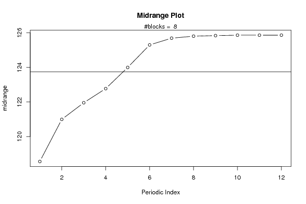
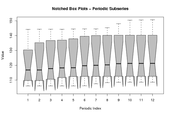
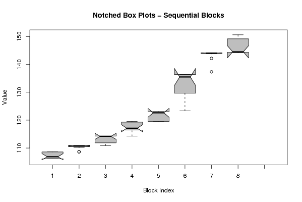
Figures (Output of Computation) | |||||||||||||||||||||
Input Parameters & R Code | |||||||||||||||||||||
| Parameters (Session): | |||||||||||||||||||||
| par1 = 12 ; | |||||||||||||||||||||
| Parameters (R input): | |||||||||||||||||||||
| par1 = 12 ; | |||||||||||||||||||||
| R code (references can be found in the software module): | |||||||||||||||||||||
par1 <- as.numeric(par1) | |||||||||||||||||||||