Repository of Reproducible Computations

Free Statistics

of Irreproducible Research!

Author's title

Author

*Unverified author*

R Software Module

rwasp_autocorrelation.wasp

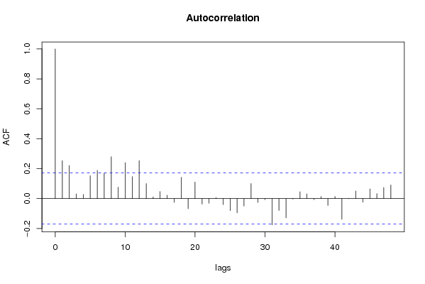
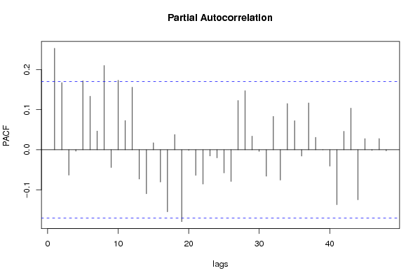
Title produced by software

(Partial) Autocorrelation Function

Date of computation

Thu, 16 Jul 2009 03:26:06 -0600

Cite this page as follows

Statistical Computations at FreeStatistics.org, Office for Research Development and Education, URL https://freestatistics.org/blog/index.php?v=date/2009/Jul/16/t12477364294kvxiqa86cz0gcx.htm/, Retrieved Fri, 24 May 2024 08:08:16 +0000

Statistical Computations at FreeStatistics.org, Office for Research Development and Education, URL https://freestatistics.org/blog/index.php?pk=42370, Retrieved Fri, 24 May 2024 08:08:16 +0000

QR Codes:

Paste this QR Code to cite your computation.

Original text written by user:

IsPrivate?

No (this computation is public)

User-defined keywords

Estimated Impact

222

Family? (F = Feedback message, R = changed R code, M = changed R Module, P = changed Parameters, D = changed Data)

-       [(Partial) Autocorrelation Function] [opgave6_autocorr_...] [2009-07-16 09:26:06] [0d1085ed835696cdd537ad5fa07600ec] [Current]

Feedback Forum

Post a new message

Dataseries X:

Download CSV

Histogram

Boxplots

0,88
1,03
0,69
0,71
1,11
1,05
1,03
0,65
0,59
0,77
0,9
1,26
0,96
0,83
0,87
0,79
1,12
0,88
0,64
0,64
0,58
0,5
0,99
1,07
0,89
0,89
0,83
0,86
0,9
1,12
0,88
0,88
0,89
0,82
0,88
0,81
0,88
0,76
1,13
0,85
1,45
1,55
0,71
0,81
0,83
0,73
0,9
0,94
1,78
0,88
1,04
0,83
1,41
0,96
1,3
0,83
1,4
0,91
0,87
0,97
1,19
1,23
1,33
1,17
1,09
0,63
0,89
0,63
1,51
0,97
0,84
0,92
0,95
0,73
1,02
0,79
1,27
0,95
0,75
0,52
0,95
0,82
0,76
1,24
0,94
1,04
1,81
0,95
1,39
0,86
1,15
1,51
0,6
0,72
1,1
1,62
1,84
1,73
1,36
1,07
1
1,49
0,9
1,43
1,54
0,81
1,61
1,3
1,4
1,03
0,79
1,11
1,15
1,03
1,59
1,11
1,33
0,93
1,07
1,14
1,12
0,86
0,82
1,02
1,07
1,31
0,98
0,89
0,8
0,8
0,78
0,97

Summary of computational transaction
Raw Input	view raw input (R code)
Raw Output	view raw output of R engine
Computing time	3 seconds
R Server	'Gwilym Jenkins' @ 72.249.127.135

\begin{tabular}{lllllllll}
\hline
Summary of computational transaction \tabularnewline
Raw Input & view raw input (R code)  \tabularnewline
Raw Output & view raw output of R engine  \tabularnewline
Computing time & 3 seconds \tabularnewline
R Server & 'Gwilym Jenkins' @ 72.249.127.135 \tabularnewline
\hline
\end{tabular}
%Source: https://freestatistics.org/blog/index.php?pk=42370&T=0

[TABLE]
[ROW][C]Summary of computational transaction[/C][/ROW]
[ROW][C]Raw Input[/C][C]view raw input (R code) [/C][/ROW]
[ROW][C]Raw Output[/C][C]view raw output of R engine [/C][/ROW]
[ROW][C]Computing time[/C][C]3 seconds[/C][/ROW]
[ROW][C]R Server[/C][C]'Gwilym Jenkins' @ 72.249.127.135[/C][/ROW]
[/TABLE]
Source: https://freestatistics.org/blog/index.php?pk=42370&T=0

Globally Unique Identifier (entire table): ba.freestatistics.org/blog/index.php?pk=42370&T=0

As an alternative you can also use a QR Code:

The GUIDs for individual cells are displayed in the table below:

Summary of computational transaction
Raw Input	view raw input (R code)
Raw Output	view raw output of R engine
Computing time	3 seconds
R Server	'Gwilym Jenkins' @ 72.249.127.135

Autocorrelation Function
Time lag k	ACF(k)	T-STAT	P-value
1	0.25355	2.9131	0.002102
2	0.221061	2.5398	0.006125
3	0.031487	0.3618	0.359054
4	0.027686	0.3181	0.375459
5	0.153114	1.7591	0.040435
6	0.188387	2.1644	0.016117
7	0.169147	1.9433	0.027051
8	0.279859	3.2153	0.000819
9	0.076396	0.8777	0.190843
10	0.24021	2.7598	0.003303
11	0.146829	1.6869	0.046989
12	0.253533	2.9129	0.002103
13	0.100301	1.1524	0.125626
14	0.010699	0.1229	0.451179
15	0.047303	0.5435	0.29386
16	0.022118	0.2541	0.3999
17	-0.02556	-0.2937	0.384737
18	0.141442	1.625	0.053269
19	-0.06768	-0.7776	0.219102
20	0.109972	1.2635	0.104321
21	-0.036732	-0.422	0.336848
22	-0.030874	-0.3547	0.361685
23	0.00707	0.0812	0.467692
24	-0.040455	-0.4648	0.321423
25	-0.081596	-0.9375	0.175116
26	-0.095634	-1.0987	0.136939
27	-0.050041	-0.5749	0.28316
28	0.100189	1.1511	0.12589
29	-0.026415	-0.3035	0.381
30	-0.007573	-0.087	0.4654
31	-0.17565	-2.0181	0.022806
32	-0.080012	-0.9193	0.179815
33	-0.128928	-1.4813	0.070459
34	-0.003583	-0.0412	0.483611
35	0.045429	0.5219	0.301295
36	0.031237	0.3589	0.360126
37	-0.008095	-0.093	0.463023
38	0.013706	0.1575	0.437558
39	-0.046496	-0.5342	0.297051
40	0.013987	0.1607	0.43629
41	-0.13855	-1.5918	0.056909
42	-0.001652	-0.019	0.492443
43	0.05101	0.5861	0.279419
44	-0.024375	-0.28	0.389941
45	0.064376	0.7396	0.230419
46	0.03307	0.3799	0.352299
47	0.074046	0.8507	0.198232
48	0.090351	1.0381	0.150571

\begin{tabular}{lllllllll}
\hline
Autocorrelation Function \tabularnewline
Time lag k & ACF(k) & T-STAT & P-value \tabularnewline
1 & 0.25355 & 2.9131 & 0.002102 \tabularnewline
2 & 0.221061 & 2.5398 & 0.006125 \tabularnewline
3 & 0.031487 & 0.3618 & 0.359054 \tabularnewline
4 & 0.027686 & 0.3181 & 0.375459 \tabularnewline
5 & 0.153114 & 1.7591 & 0.040435 \tabularnewline
6 & 0.188387 & 2.1644 & 0.016117 \tabularnewline
7 & 0.169147 & 1.9433 & 0.027051 \tabularnewline
8 & 0.279859 & 3.2153 & 0.000819 \tabularnewline
9 & 0.076396 & 0.8777 & 0.190843 \tabularnewline
10 & 0.24021 & 2.7598 & 0.003303 \tabularnewline
11 & 0.146829 & 1.6869 & 0.046989 \tabularnewline
12 & 0.253533 & 2.9129 & 0.002103 \tabularnewline
13 & 0.100301 & 1.1524 & 0.125626 \tabularnewline
14 & 0.010699 & 0.1229 & 0.451179 \tabularnewline
15 & 0.047303 & 0.5435 & 0.29386 \tabularnewline
16 & 0.022118 & 0.2541 & 0.3999 \tabularnewline
17 & -0.02556 & -0.2937 & 0.384737 \tabularnewline
18 & 0.141442 & 1.625 & 0.053269 \tabularnewline
19 & -0.06768 & -0.7776 & 0.219102 \tabularnewline
20 & 0.109972 & 1.2635 & 0.104321 \tabularnewline
21 & -0.036732 & -0.422 & 0.336848 \tabularnewline
22 & -0.030874 & -0.3547 & 0.361685 \tabularnewline
23 & 0.00707 & 0.0812 & 0.467692 \tabularnewline
24 & -0.040455 & -0.4648 & 0.321423 \tabularnewline
25 & -0.081596 & -0.9375 & 0.175116 \tabularnewline
26 & -0.095634 & -1.0987 & 0.136939 \tabularnewline
27 & -0.050041 & -0.5749 & 0.28316 \tabularnewline
28 & 0.100189 & 1.1511 & 0.12589 \tabularnewline
29 & -0.026415 & -0.3035 & 0.381 \tabularnewline
30 & -0.007573 & -0.087 & 0.4654 \tabularnewline
31 & -0.17565 & -2.0181 & 0.022806 \tabularnewline
32 & -0.080012 & -0.9193 & 0.179815 \tabularnewline
33 & -0.128928 & -1.4813 & 0.070459 \tabularnewline
34 & -0.003583 & -0.0412 & 0.483611 \tabularnewline
35 & 0.045429 & 0.5219 & 0.301295 \tabularnewline
36 & 0.031237 & 0.3589 & 0.360126 \tabularnewline
37 & -0.008095 & -0.093 & 0.463023 \tabularnewline
38 & 0.013706 & 0.1575 & 0.437558 \tabularnewline
39 & -0.046496 & -0.5342 & 0.297051 \tabularnewline
40 & 0.013987 & 0.1607 & 0.43629 \tabularnewline
41 & -0.13855 & -1.5918 & 0.056909 \tabularnewline
42 & -0.001652 & -0.019 & 0.492443 \tabularnewline
43 & 0.05101 & 0.5861 & 0.279419 \tabularnewline
44 & -0.024375 & -0.28 & 0.389941 \tabularnewline
45 & 0.064376 & 0.7396 & 0.230419 \tabularnewline
46 & 0.03307 & 0.3799 & 0.352299 \tabularnewline
47 & 0.074046 & 0.8507 & 0.198232 \tabularnewline
48 & 0.090351 & 1.0381 & 0.150571 \tabularnewline
\hline
\end{tabular}
%Source: https://freestatistics.org/blog/index.php?pk=42370&T=1

[TABLE]
[ROW][C]Autocorrelation Function[/C][/ROW]
[ROW][C]Time lag k[/C][C]ACF(k)[/C][C]T-STAT[/C][C]P-value[/C][/ROW]
[ROW][C]1[/C][C]0.25355[/C][C]2.9131[/C][C]0.002102[/C][/ROW]
[ROW][C]2[/C][C]0.221061[/C][C]2.5398[/C][C]0.006125[/C][/ROW]
[ROW][C]3[/C][C]0.031487[/C][C]0.3618[/C][C]0.359054[/C][/ROW]
[ROW][C]4[/C][C]0.027686[/C][C]0.3181[/C][C]0.375459[/C][/ROW]
[ROW][C]5[/C][C]0.153114[/C][C]1.7591[/C][C]0.040435[/C][/ROW]
[ROW][C]6[/C][C]0.188387[/C][C]2.1644[/C][C]0.016117[/C][/ROW]
[ROW][C]7[/C][C]0.169147[/C][C]1.9433[/C][C]0.027051[/C][/ROW]
[ROW][C]8[/C][C]0.279859[/C][C]3.2153[/C][C]0.000819[/C][/ROW]
[ROW][C]9[/C][C]0.076396[/C][C]0.8777[/C][C]0.190843[/C][/ROW]
[ROW][C]10[/C][C]0.24021[/C][C]2.7598[/C][C]0.003303[/C][/ROW]
[ROW][C]11[/C][C]0.146829[/C][C]1.6869[/C][C]0.046989[/C][/ROW]
[ROW][C]12[/C][C]0.253533[/C][C]2.9129[/C][C]0.002103[/C][/ROW]
[ROW][C]13[/C][C]0.100301[/C][C]1.1524[/C][C]0.125626[/C][/ROW]
[ROW][C]14[/C][C]0.010699[/C][C]0.1229[/C][C]0.451179[/C][/ROW]
[ROW][C]15[/C][C]0.047303[/C][C]0.5435[/C][C]0.29386[/C][/ROW]
[ROW][C]16[/C][C]0.022118[/C][C]0.2541[/C][C]0.3999[/C][/ROW]
[ROW][C]17[/C][C]-0.02556[/C][C]-0.2937[/C][C]0.384737[/C][/ROW]
[ROW][C]18[/C][C]0.141442[/C][C]1.625[/C][C]0.053269[/C][/ROW]
[ROW][C]19[/C][C]-0.06768[/C][C]-0.7776[/C][C]0.219102[/C][/ROW]
[ROW][C]20[/C][C]0.109972[/C][C]1.2635[/C][C]0.104321[/C][/ROW]
[ROW][C]21[/C][C]-0.036732[/C][C]-0.422[/C][C]0.336848[/C][/ROW]
[ROW][C]22[/C][C]-0.030874[/C][C]-0.3547[/C][C]0.361685[/C][/ROW]
[ROW][C]23[/C][C]0.00707[/C][C]0.0812[/C][C]0.467692[/C][/ROW]
[ROW][C]24[/C][C]-0.040455[/C][C]-0.4648[/C][C]0.321423[/C][/ROW]
[ROW][C]25[/C][C]-0.081596[/C][C]-0.9375[/C][C]0.175116[/C][/ROW]
[ROW][C]26[/C][C]-0.095634[/C][C]-1.0987[/C][C]0.136939[/C][/ROW]
[ROW][C]27[/C][C]-0.050041[/C][C]-0.5749[/C][C]0.28316[/C][/ROW]
[ROW][C]28[/C][C]0.100189[/C][C]1.1511[/C][C]0.12589[/C][/ROW]
[ROW][C]29[/C][C]-0.026415[/C][C]-0.3035[/C][C]0.381[/C][/ROW]
[ROW][C]30[/C][C]-0.007573[/C][C]-0.087[/C][C]0.4654[/C][/ROW]
[ROW][C]31[/C][C]-0.17565[/C][C]-2.0181[/C][C]0.022806[/C][/ROW]
[ROW][C]32[/C][C]-0.080012[/C][C]-0.9193[/C][C]0.179815[/C][/ROW]
[ROW][C]33[/C][C]-0.128928[/C][C]-1.4813[/C][C]0.070459[/C][/ROW]
[ROW][C]34[/C][C]-0.003583[/C][C]-0.0412[/C][C]0.483611[/C][/ROW]
[ROW][C]35[/C][C]0.045429[/C][C]0.5219[/C][C]0.301295[/C][/ROW]
[ROW][C]36[/C][C]0.031237[/C][C]0.3589[/C][C]0.360126[/C][/ROW]
[ROW][C]37[/C][C]-0.008095[/C][C]-0.093[/C][C]0.463023[/C][/ROW]
[ROW][C]38[/C][C]0.013706[/C][C]0.1575[/C][C]0.437558[/C][/ROW]
[ROW][C]39[/C][C]-0.046496[/C][C]-0.5342[/C][C]0.297051[/C][/ROW]
[ROW][C]40[/C][C]0.013987[/C][C]0.1607[/C][C]0.43629[/C][/ROW]
[ROW][C]41[/C][C]-0.13855[/C][C]-1.5918[/C][C]0.056909[/C][/ROW]
[ROW][C]42[/C][C]-0.001652[/C][C]-0.019[/C][C]0.492443[/C][/ROW]
[ROW][C]43[/C][C]0.05101[/C][C]0.5861[/C][C]0.279419[/C][/ROW]
[ROW][C]44[/C][C]-0.024375[/C][C]-0.28[/C][C]0.389941[/C][/ROW]
[ROW][C]45[/C][C]0.064376[/C][C]0.7396[/C][C]0.230419[/C][/ROW]
[ROW][C]46[/C][C]0.03307[/C][C]0.3799[/C][C]0.352299[/C][/ROW]
[ROW][C]47[/C][C]0.074046[/C][C]0.8507[/C][C]0.198232[/C][/ROW]
[ROW][C]48[/C][C]0.090351[/C][C]1.0381[/C][C]0.150571[/C][/ROW]
[/TABLE]
Source: https://freestatistics.org/blog/index.php?pk=42370&T=1

Globally Unique Identifier (entire table): ba.freestatistics.org/blog/index.php?pk=42370&T=1

As an alternative you can also use a QR Code:

The GUIDs for individual cells are displayed in the table below:

Autocorrelation Function
Time lag k	ACF(k)	T-STAT	P-value
1	0.25355	2.9131	0.002102
2	0.221061	2.5398	0.006125
3	0.031487	0.3618	0.359054
4	0.027686	0.3181	0.375459
5	0.153114	1.7591	0.040435
6	0.188387	2.1644	0.016117
7	0.169147	1.9433	0.027051
8	0.279859	3.2153	0.000819
9	0.076396	0.8777	0.190843
10	0.24021	2.7598	0.003303
11	0.146829	1.6869	0.046989
12	0.253533	2.9129	0.002103
13	0.100301	1.1524	0.125626
14	0.010699	0.1229	0.451179
15	0.047303	0.5435	0.29386
16	0.022118	0.2541	0.3999
17	-0.02556	-0.2937	0.384737
18	0.141442	1.625	0.053269
19	-0.06768	-0.7776	0.219102
20	0.109972	1.2635	0.104321
21	-0.036732	-0.422	0.336848
22	-0.030874	-0.3547	0.361685
23	0.00707	0.0812	0.467692
24	-0.040455	-0.4648	0.321423
25	-0.081596	-0.9375	0.175116
26	-0.095634	-1.0987	0.136939
27	-0.050041	-0.5749	0.28316
28	0.100189	1.1511	0.12589
29	-0.026415	-0.3035	0.381
30	-0.007573	-0.087	0.4654
31	-0.17565	-2.0181	0.022806
32	-0.080012	-0.9193	0.179815
33	-0.128928	-1.4813	0.070459
34	-0.003583	-0.0412	0.483611
35	0.045429	0.5219	0.301295
36	0.031237	0.3589	0.360126
37	-0.008095	-0.093	0.463023
38	0.013706	0.1575	0.437558
39	-0.046496	-0.5342	0.297051
40	0.013987	0.1607	0.43629
41	-0.13855	-1.5918	0.056909
42	-0.001652	-0.019	0.492443
43	0.05101	0.5861	0.279419
44	-0.024375	-0.28	0.389941
45	0.064376	0.7396	0.230419
46	0.03307	0.3799	0.352299
47	0.074046	0.8507	0.198232
48	0.090351	1.0381	0.150571

Partial Autocorrelation Function
Time lag k	PACF(k)	T-STAT	P-value
1	0.25355	2.9131	0.002102
2	0.167545	1.9249	0.028194
3	-0.063394	-0.7283	0.233849
4	-0.003551	-0.0408	0.48376
5	0.172233	1.9788	0.024959
6	0.133758	1.5368	0.063372
7	0.046685	0.5364	0.296305
8	0.210608	2.4197	0.008447
9	-0.04442	-0.5103	0.305331
10	0.173462	1.9929	0.024166
11	0.072996	0.8387	0.201589
12	0.15618	1.7944	0.037521
13	-0.073299	-0.8421	0.200616
14	-0.110034	-1.2642	0.104194
15	0.017447	0.2005	0.420719
16	-0.080717	-0.9274	0.177715
17	-0.155109	-1.7821	0.038519
18	0.037996	0.4365	0.331578
19	-0.179697	-2.0646	0.020461
20	-0.001316	-0.0151	0.49398
21	-0.063818	-0.7332	0.232365
22	-0.085841	-0.9862	0.162909
23	-0.015589	-0.1791	0.429065
24	-0.02045	-0.235	0.407305
25	-0.057972	-0.666	0.253271
26	-0.079088	-0.9087	0.182595
27	0.122991	1.4131	0.079996
28	0.147562	1.6954	0.046182
29	0.034058	0.3913	0.348105
30	-0.0039	-0.0448	0.482163
31	-0.066184	-0.7604	0.224187
32	0.083207	0.956	0.170417
33	-0.076016	-0.8734	0.192027
34	0.115424	1.3261	0.093545
35	0.072486	0.8328	0.20323
36	-0.015768	-0.1812	0.428262
37	0.116826	1.3422	0.090914
38	0.03091	0.3551	0.361528
39	0.000291	0.0033	0.498669
40	-0.040852	-0.4694	0.319795
41	-0.137239	-1.5768	0.058623
42	0.046006	0.5286	0.298998
43	0.104038	1.1953	0.117055
44	-0.125028	-1.4365	0.076618
45	0.027795	0.3193	0.374986
46	-0.001487	-0.0171	0.493199
47	0.02792	0.3208	0.374442
48	-0.002605	-0.0299	0.488083

\begin{tabular}{lllllllll}
\hline
Partial Autocorrelation Function \tabularnewline
Time lag k & PACF(k) & T-STAT & P-value \tabularnewline
1 & 0.25355 & 2.9131 & 0.002102 \tabularnewline
2 & 0.167545 & 1.9249 & 0.028194 \tabularnewline
3 & -0.063394 & -0.7283 & 0.233849 \tabularnewline
4 & -0.003551 & -0.0408 & 0.48376 \tabularnewline
5 & 0.172233 & 1.9788 & 0.024959 \tabularnewline
6 & 0.133758 & 1.5368 & 0.063372 \tabularnewline
7 & 0.046685 & 0.5364 & 0.296305 \tabularnewline
8 & 0.210608 & 2.4197 & 0.008447 \tabularnewline
9 & -0.04442 & -0.5103 & 0.305331 \tabularnewline
10 & 0.173462 & 1.9929 & 0.024166 \tabularnewline
11 & 0.072996 & 0.8387 & 0.201589 \tabularnewline
12 & 0.15618 & 1.7944 & 0.037521 \tabularnewline
13 & -0.073299 & -0.8421 & 0.200616 \tabularnewline
14 & -0.110034 & -1.2642 & 0.104194 \tabularnewline
15 & 0.017447 & 0.2005 & 0.420719 \tabularnewline
16 & -0.080717 & -0.9274 & 0.177715 \tabularnewline
17 & -0.155109 & -1.7821 & 0.038519 \tabularnewline
18 & 0.037996 & 0.4365 & 0.331578 \tabularnewline
19 & -0.179697 & -2.0646 & 0.020461 \tabularnewline
20 & -0.001316 & -0.0151 & 0.49398 \tabularnewline
21 & -0.063818 & -0.7332 & 0.232365 \tabularnewline
22 & -0.085841 & -0.9862 & 0.162909 \tabularnewline
23 & -0.015589 & -0.1791 & 0.429065 \tabularnewline
24 & -0.02045 & -0.235 & 0.407305 \tabularnewline
25 & -0.057972 & -0.666 & 0.253271 \tabularnewline
26 & -0.079088 & -0.9087 & 0.182595 \tabularnewline
27 & 0.122991 & 1.4131 & 0.079996 \tabularnewline
28 & 0.147562 & 1.6954 & 0.046182 \tabularnewline
29 & 0.034058 & 0.3913 & 0.348105 \tabularnewline
30 & -0.0039 & -0.0448 & 0.482163 \tabularnewline
31 & -0.066184 & -0.7604 & 0.224187 \tabularnewline
32 & 0.083207 & 0.956 & 0.170417 \tabularnewline
33 & -0.076016 & -0.8734 & 0.192027 \tabularnewline
34 & 0.115424 & 1.3261 & 0.093545 \tabularnewline
35 & 0.072486 & 0.8328 & 0.20323 \tabularnewline
36 & -0.015768 & -0.1812 & 0.428262 \tabularnewline
37 & 0.116826 & 1.3422 & 0.090914 \tabularnewline
38 & 0.03091 & 0.3551 & 0.361528 \tabularnewline
39 & 0.000291 & 0.0033 & 0.498669 \tabularnewline
40 & -0.040852 & -0.4694 & 0.319795 \tabularnewline
41 & -0.137239 & -1.5768 & 0.058623 \tabularnewline
42 & 0.046006 & 0.5286 & 0.298998 \tabularnewline
43 & 0.104038 & 1.1953 & 0.117055 \tabularnewline
44 & -0.125028 & -1.4365 & 0.076618 \tabularnewline
45 & 0.027795 & 0.3193 & 0.374986 \tabularnewline
46 & -0.001487 & -0.0171 & 0.493199 \tabularnewline
47 & 0.02792 & 0.3208 & 0.374442 \tabularnewline
48 & -0.002605 & -0.0299 & 0.488083 \tabularnewline
\hline
\end{tabular}
%Source: https://freestatistics.org/blog/index.php?pk=42370&T=2

[TABLE]
[ROW][C]Partial Autocorrelation Function[/C][/ROW]
[ROW][C]Time lag k[/C][C]PACF(k)[/C][C]T-STAT[/C][C]P-value[/C][/ROW]
[ROW][C]1[/C][C]0.25355[/C][C]2.9131[/C][C]0.002102[/C][/ROW]
[ROW][C]2[/C][C]0.167545[/C][C]1.9249[/C][C]0.028194[/C][/ROW]
[ROW][C]3[/C][C]-0.063394[/C][C]-0.7283[/C][C]0.233849[/C][/ROW]
[ROW][C]4[/C][C]-0.003551[/C][C]-0.0408[/C][C]0.48376[/C][/ROW]
[ROW][C]5[/C][C]0.172233[/C][C]1.9788[/C][C]0.024959[/C][/ROW]
[ROW][C]6[/C][C]0.133758[/C][C]1.5368[/C][C]0.063372[/C][/ROW]
[ROW][C]7[/C][C]0.046685[/C][C]0.5364[/C][C]0.296305[/C][/ROW]
[ROW][C]8[/C][C]0.210608[/C][C]2.4197[/C][C]0.008447[/C][/ROW]
[ROW][C]9[/C][C]-0.04442[/C][C]-0.5103[/C][C]0.305331[/C][/ROW]
[ROW][C]10[/C][C]0.173462[/C][C]1.9929[/C][C]0.024166[/C][/ROW]
[ROW][C]11[/C][C]0.072996[/C][C]0.8387[/C][C]0.201589[/C][/ROW]
[ROW][C]12[/C][C]0.15618[/C][C]1.7944[/C][C]0.037521[/C][/ROW]
[ROW][C]13[/C][C]-0.073299[/C][C]-0.8421[/C][C]0.200616[/C][/ROW]
[ROW][C]14[/C][C]-0.110034[/C][C]-1.2642[/C][C]0.104194[/C][/ROW]
[ROW][C]15[/C][C]0.017447[/C][C]0.2005[/C][C]0.420719[/C][/ROW]
[ROW][C]16[/C][C]-0.080717[/C][C]-0.9274[/C][C]0.177715[/C][/ROW]
[ROW][C]17[/C][C]-0.155109[/C][C]-1.7821[/C][C]0.038519[/C][/ROW]
[ROW][C]18[/C][C]0.037996[/C][C]0.4365[/C][C]0.331578[/C][/ROW]
[ROW][C]19[/C][C]-0.179697[/C][C]-2.0646[/C][C]0.020461[/C][/ROW]
[ROW][C]20[/C][C]-0.001316[/C][C]-0.0151[/C][C]0.49398[/C][/ROW]
[ROW][C]21[/C][C]-0.063818[/C][C]-0.7332[/C][C]0.232365[/C][/ROW]
[ROW][C]22[/C][C]-0.085841[/C][C]-0.9862[/C][C]0.162909[/C][/ROW]
[ROW][C]23[/C][C]-0.015589[/C][C]-0.1791[/C][C]0.429065[/C][/ROW]
[ROW][C]24[/C][C]-0.02045[/C][C]-0.235[/C][C]0.407305[/C][/ROW]
[ROW][C]25[/C][C]-0.057972[/C][C]-0.666[/C][C]0.253271[/C][/ROW]
[ROW][C]26[/C][C]-0.079088[/C][C]-0.9087[/C][C]0.182595[/C][/ROW]
[ROW][C]27[/C][C]0.122991[/C][C]1.4131[/C][C]0.079996[/C][/ROW]
[ROW][C]28[/C][C]0.147562[/C][C]1.6954[/C][C]0.046182[/C][/ROW]
[ROW][C]29[/C][C]0.034058[/C][C]0.3913[/C][C]0.348105[/C][/ROW]
[ROW][C]30[/C][C]-0.0039[/C][C]-0.0448[/C][C]0.482163[/C][/ROW]
[ROW][C]31[/C][C]-0.066184[/C][C]-0.7604[/C][C]0.224187[/C][/ROW]
[ROW][C]32[/C][C]0.083207[/C][C]0.956[/C][C]0.170417[/C][/ROW]
[ROW][C]33[/C][C]-0.076016[/C][C]-0.8734[/C][C]0.192027[/C][/ROW]
[ROW][C]34[/C][C]0.115424[/C][C]1.3261[/C][C]0.093545[/C][/ROW]
[ROW][C]35[/C][C]0.072486[/C][C]0.8328[/C][C]0.20323[/C][/ROW]
[ROW][C]36[/C][C]-0.015768[/C][C]-0.1812[/C][C]0.428262[/C][/ROW]
[ROW][C]37[/C][C]0.116826[/C][C]1.3422[/C][C]0.090914[/C][/ROW]
[ROW][C]38[/C][C]0.03091[/C][C]0.3551[/C][C]0.361528[/C][/ROW]
[ROW][C]39[/C][C]0.000291[/C][C]0.0033[/C][C]0.498669[/C][/ROW]
[ROW][C]40[/C][C]-0.040852[/C][C]-0.4694[/C][C]0.319795[/C][/ROW]
[ROW][C]41[/C][C]-0.137239[/C][C]-1.5768[/C][C]0.058623[/C][/ROW]
[ROW][C]42[/C][C]0.046006[/C][C]0.5286[/C][C]0.298998[/C][/ROW]
[ROW][C]43[/C][C]0.104038[/C][C]1.1953[/C][C]0.117055[/C][/ROW]
[ROW][C]44[/C][C]-0.125028[/C][C]-1.4365[/C][C]0.076618[/C][/ROW]
[ROW][C]45[/C][C]0.027795[/C][C]0.3193[/C][C]0.374986[/C][/ROW]
[ROW][C]46[/C][C]-0.001487[/C][C]-0.0171[/C][C]0.493199[/C][/ROW]
[ROW][C]47[/C][C]0.02792[/C][C]0.3208[/C][C]0.374442[/C][/ROW]
[ROW][C]48[/C][C]-0.002605[/C][C]-0.0299[/C][C]0.488083[/C][/ROW]
[/TABLE]
Source: https://freestatistics.org/blog/index.php?pk=42370&T=2

Globally Unique Identifier (entire table): ba.freestatistics.org/blog/index.php?pk=42370&T=2

As an alternative you can also use a QR Code:

The GUIDs for individual cells are displayed in the table below:

Partial Autocorrelation Function
Time lag k	PACF(k)	T-STAT	P-value
1	0.25355	2.9131	0.002102
2	0.167545	1.9249	0.028194
3	-0.063394	-0.7283	0.233849
4	-0.003551	-0.0408	0.48376
5	0.172233	1.9788	0.024959
6	0.133758	1.5368	0.063372
7	0.046685	0.5364	0.296305
8	0.210608	2.4197	0.008447
9	-0.04442	-0.5103	0.305331
10	0.173462	1.9929	0.024166
11	0.072996	0.8387	0.201589
12	0.15618	1.7944	0.037521
13	-0.073299	-0.8421	0.200616
14	-0.110034	-1.2642	0.104194
15	0.017447	0.2005	0.420719
16	-0.080717	-0.9274	0.177715
17	-0.155109	-1.7821	0.038519
18	0.037996	0.4365	0.331578
19	-0.179697	-2.0646	0.020461
20	-0.001316	-0.0151	0.49398
21	-0.063818	-0.7332	0.232365
22	-0.085841	-0.9862	0.162909
23	-0.015589	-0.1791	0.429065
24	-0.02045	-0.235	0.407305
25	-0.057972	-0.666	0.253271
26	-0.079088	-0.9087	0.182595
27	0.122991	1.4131	0.079996
28	0.147562	1.6954	0.046182
29	0.034058	0.3913	0.348105
30	-0.0039	-0.0448	0.482163
31	-0.066184	-0.7604	0.224187
32	0.083207	0.956	0.170417
33	-0.076016	-0.8734	0.192027
34	0.115424	1.3261	0.093545
35	0.072486	0.8328	0.20323
36	-0.015768	-0.1812	0.428262
37	0.116826	1.3422	0.090914
38	0.03091	0.3551	0.361528
39	0.000291	0.0033	0.498669
40	-0.040852	-0.4694	0.319795
41	-0.137239	-1.5768	0.058623
42	0.046006	0.5286	0.298998
43	0.104038	1.1953	0.117055
44	-0.125028	-1.4365	0.076618
45	0.027795	0.3193	0.374986
46	-0.001487	-0.0171	0.493199
47	0.02792	0.3208	0.374442
48	-0.002605	-0.0299	0.488083

Figure 1

PNG link

Postscript link

PDF link

Figure 2

PNG link

Postscript link

PDF link

Parameters (Session):

par1 = 48 ; par2 = 1 ; par3 = 0 ; par4 = 0 ; par5 = 12 ;

Parameters (R input):

par1 = 48 ; par2 = 1 ; par3 = 0 ; par4 = 0 ; par5 = 12 ;

R code (references can be found in the software module):

if (par1 == 'Default') {
par1 = 10*log10(length(x))
} else {
par1 <- as.numeric(par1)
}
par2 <- as.numeric(par2)
par3 <- as.numeric(par3)
par4 <- as.numeric(par4)
par5 <- as.numeric(par5)
if (par2 == 0) {
x <- log(x)
} else {
x <- (x ^ par2 - 1) / par2
}
if (par3 > 0) x <- diff(x,lag=1,difference=par3)
if (par4 > 0) x <- diff(x,lag=par5,difference=par4)
bitmap(file='pic1.png')
racf <- acf(x,par1,main='Autocorrelation',xlab='lags',ylab='ACF')
dev.off()
bitmap(file='pic2.png')
rpacf <- pacf(x,par1,main='Partial Autocorrelation',xlab='lags',ylab='PACF')
dev.off()
(myacf <- c(racf$acf))
(mypacf <- c(rpacf$acf))
lengthx <- length(x)
sqrtn <- sqrt(lengthx)
load(file='createtable')
a<-table.start()
a<-table.row.start(a)
a<-table.element(a,'Autocorrelation Function',4,TRUE)
a<-table.row.end(a)
a<-table.row.start(a)
a<-table.element(a,'Time lag k',header=TRUE)
a<-table.element(a,hyperlink('basics.htm','ACF(k)','click here for more information about the Autocorrelation Function'),header=TRUE)
a<-table.element(a,'T-STAT',header=TRUE)
a<-table.element(a,'P-value',header=TRUE)
a<-table.row.end(a)
for (i in 2:(par1+1)) {
a<-table.row.start(a)
a<-table.element(a,i-1,header=TRUE)
a<-table.element(a,round(myacf[i],6))
mytstat <- myacf[i]*sqrtn
a<-table.element(a,round(mytstat,4))
a<-table.element(a,round(1-pt(abs(mytstat),lengthx),6))
a<-table.row.end(a)
}
a<-table.end(a)
table.save(a,file='mytable.tab')
a<-table.start()
a<-table.row.start(a)
a<-table.element(a,'Partial Autocorrelation Function',4,TRUE)
a<-table.row.end(a)
a<-table.row.start(a)
a<-table.element(a,'Time lag k',header=TRUE)
a<-table.element(a,hyperlink('basics.htm','PACF(k)','click here for more information about the Partial Autocorrelation Function'),header=TRUE)
a<-table.element(a,'T-STAT',header=TRUE)
a<-table.element(a,'P-value',header=TRUE)
a<-table.row.end(a)
for (i in 1:par1) {
a<-table.row.start(a)
a<-table.element(a,i,header=TRUE)
a<-table.element(a,round(mypacf[i],6))
mytstat <- mypacf[i]*sqrtn
a<-table.element(a,round(mytstat,4))
a<-table.element(a,round(1-pt(abs(mytstat),lengthx),6))
a<-table.row.end(a)
}
a<-table.end(a)
table.save(a,file='mytable1.tab')

Free Statistics

Description of Statistical Computation

Tree of Dependent Computations

Dataset

Tables (Output of Computation)

Figures (Output of Computation)

Input Parameters & R Code