Free Statistics
of Irreproducible Research!
Description of Statistical Computation | |||||||||||||||||||||
|---|---|---|---|---|---|---|---|---|---|---|---|---|---|---|---|---|---|---|---|---|---|
| Author's title | |||||||||||||||||||||
| Author | *The author of this computation has been verified* | ||||||||||||||||||||
| R Software Module | rwasp_meanplot.wasp | ||||||||||||||||||||
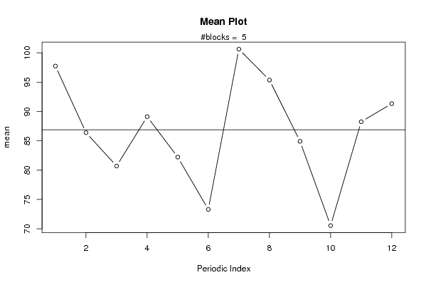
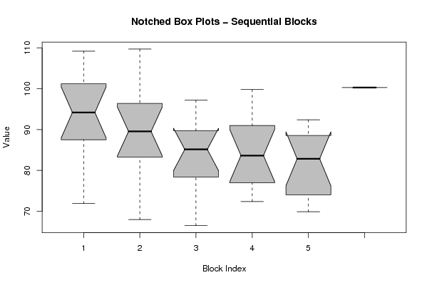
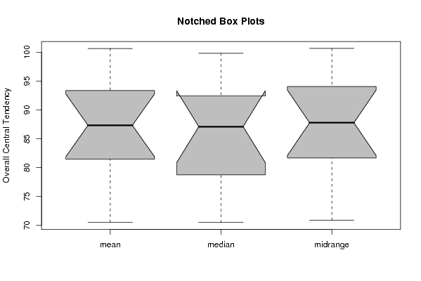
| Title produced by software | Mean Plot | ||||||||||||||||||||
| Date of computation | Fri, 31 Oct 2008 03:40:26 -0600 | ||||||||||||||||||||
| Cite this page as follows | Statistical Computations at FreeStatistics.org, Office for Research Development and Education, URL https://freestatistics.org/blog/index.php?v=date/2008/Oct/31/t12254461034ff8vhuj35jv56c.htm/, Retrieved Sun, 19 May 2024 15:23:58 +0000 | ||||||||||||||||||||
| Statistical Computations at FreeStatistics.org, Office for Research Development and Education, URL https://freestatistics.org/blog/index.php?pk=20199, Retrieved Sun, 19 May 2024 15:23:58 +0000 | |||||||||||||||||||||
| QR Codes: | |||||||||||||||||||||
|
| |||||||||||||||||||||
| Original text written by user: | |||||||||||||||||||||
| IsPrivate? | No (this computation is public) | ||||||||||||||||||||
| User-defined keywords | |||||||||||||||||||||
| Estimated Impact | 235 | ||||||||||||||||||||
Tree of Dependent Computations | |||||||||||||||||||||
| Family? (F = Feedback message, R = changed R code, M = changed R Module, P = changed Parameters, D = changed Data) | |||||||||||||||||||||
| F [Notched Boxplots] [workshop 3] [2007-10-26 13:31:48] [e9ffc5de6f8a7be62f22b142b5b6b1a8] F RMPD [Mean Plot] [workshop 4 deel 1...] [2008-10-31 09:40:26] [3817f5e632a8bfeb1be7b5e8c86bd450] [Current] F R [Mean Plot] [opdracht 4 task 4] [2008-10-31 13:19:40] [077ffec662d24c06be4c491541a44245] F [Mean Plot] [] [2008-11-01 13:19:15] [4c8dfb519edec2da3492d7e6be9a5685] F R [Mean Plot] [] [2008-11-01 13:59:33] [4c8dfb519edec2da3492d7e6be9a5685] F [Mean Plot] [Task 4 - Bob Leysen] [2008-11-02 15:49:09] [57850c80fd59ccfb28f882be994e814e] F [Mean Plot] [Task 4] [2008-11-02 16:04:40] [73d6180dc45497329efd1b6934a84aba] F [Mean Plot] [Task 4] [2008-11-02 19:16:07] [6816386b1f3c2f6c0c9f2aa1e5bc9362] F D [Mean Plot] [] [2008-11-01 14:24:03] [4c8dfb519edec2da3492d7e6be9a5685] F D [Mean Plot] [Task 5 - Bob Leysen] [2008-11-02 16:03:09] [57850c80fd59ccfb28f882be994e814e] F D [Mean Plot] [opdracht 4 task 5] [2008-11-03 17:56:26] [077ffec662d24c06be4c491541a44245] - D [Mean Plot] [task 5] [2008-11-02 16:22:21] [73d6180dc45497329efd1b6934a84aba] F RMPD [Star Plot] [Star Plot - Bob L...] [2008-11-02 16:44:14] [57850c80fd59ccfb28f882be994e814e] F P [Star Plot] [Q2 -part 2] [2008-11-02 18:39:32] [73d6180dc45497329efd1b6934a84aba] F P [Star Plot] [Star plot - Stefa...] [2008-11-03 19:45:53] [393f8bd7ec1141df13b2cdc1ba8ed059] - D [Star Plot] [Verbetering Q2] [2008-11-05 17:50:39] [2d4aec5ed1856c4828162be37be304d9] - [Star Plot] [Verbetering] [2008-11-09 11:11:25] [79c17183721a40a589db5f9f561947d8] - P [Star Plot] [Part 2 - Q2] [2008-11-03 19:55:23] [547636b63517c1c2916a747d66b36ebf] - P [Star Plot] [Q2- Jens Peeters] [2008-11-11 10:44:11] [b47fceb71c9525e79a89b5fc6d023d0e] F RMPD [Testing Mean with known Variance - Critical Value] [Q1] [2008-11-11 12:00:37] [b47fceb71c9525e79a89b5fc6d023d0e] F RMPD [Testing Mean with known Variance - p-value] [Q2] [2008-11-11 12:25:49] [b47fceb71c9525e79a89b5fc6d023d0e] F RMPD [Testing Mean with known Variance - Type II Error] [Q3] [2008-11-11 12:43:52] [b47fceb71c9525e79a89b5fc6d023d0e] F RMPD [Testing Mean with known Variance - Sample Size] [Q4] [2008-11-11 12:54:50] [b47fceb71c9525e79a89b5fc6d023d0e] F RMPD [Testing Population Mean with known Variance - Confidence Interval] [Q5] [2008-11-11 13:03:28] [b47fceb71c9525e79a89b5fc6d023d0e] F RMPD [Testing Sample Mean with known Variance - Confidence Interval] [Q6] [2008-11-11 13:11:57] [b47fceb71c9525e79a89b5fc6d023d0e] F RMPD [Bivariate Kernel Density Estimation] [Q1-1] [2008-11-11 14:13:42] [b47fceb71c9525e79a89b5fc6d023d0e] F RM D [Partial Correlation] [Q1-2] [2008-11-11 14:17:22] [b47fceb71c9525e79a89b5fc6d023d0e] F RMPD [Trivariate Scatterplots] [Q1-3] [2008-11-11 14:19:10] [b47fceb71c9525e79a89b5fc6d023d0e] F D [Mean Plot] [task 5] [2008-11-02 17:55:34] [73d6180dc45497329efd1b6934a84aba] F RM D [Kendall tau Correlation Matrix] [] [2008-11-01 14:54:43] [4c8dfb519edec2da3492d7e6be9a5685] F RM D [Star Plot] [] [2008-11-01 15:07:20] [4c8dfb519edec2da3492d7e6be9a5685] F RM D [Notched Boxplots] [] [2008-11-01 15:20:06] [4c8dfb519edec2da3492d7e6be9a5685] F P [Notched Boxplots] [] [2008-11-02 21:57:12] [077ffec662d24c06be4c491541a44245] F P [Star Plot] [] [2008-11-02 21:55:44] [077ffec662d24c06be4c491541a44245] F PD [Kendall tau Correlation Matrix] [] [2008-11-02 21:54:30] [077ffec662d24c06be4c491541a44245] F [Mean Plot] [Task 1 - Bob Leysen] [2008-11-02 15:25:34] [57850c80fd59ccfb28f882be994e814e] F P [Mean Plot] [] [2008-11-06 19:08:36] [072bb89749ef40809573ea0372b43d78] F [Mean Plot] [task 4 ] [2008-11-02 16:02:26] [73d6180dc45497329efd1b6934a84aba] - [Mean Plot] [Task 4] [2008-11-02 19:13:48] [6816386b1f3c2f6c0c9f2aa1e5bc9362] - P [Mean Plot] [EDA part 1 - Q4 -...] [2008-11-11 08:41:43] [33f4701c7363e8b81858dafbf0350eed] F [Mean Plot] [] [2008-11-01 13:27:58] [4c8dfb519edec2da3492d7e6be9a5685] F [Mean Plot] [] [2008-11-02 15:27:19] [57850c80fd59ccfb28f882be994e814e] - D [Mean Plot] [Hypothesis Testin...] [2008-12-08 21:24:08] [59aea967d9353ed104ab16378d373ac2] - PD [Mean Plot] [Mean plot werkloo...] [2008-12-19 15:31:03] [8b0d202c3a0c4ea223fd8b8e731dacd8] - D [Mean Plot] [Mean plot inschr ...] [2008-12-19 16:01:42] [8b0d202c3a0c4ea223fd8b8e731dacd8] | |||||||||||||||||||||
| Feedback Forum | |||||||||||||||||||||
Post a new message | |||||||||||||||||||||
Dataset | |||||||||||||||||||||
| Dataseries X: | |||||||||||||||||||||
109.20 88.60 94.30 98.30 86.40 80.60 104.10 108.20 93.40 71.90 94.10 94.90 96.40 91.10 84.40 86.40 88.00 75.10 109.70 103.00 82.10 68.00 96.40 94.30 90.00 88.00 76.10 82.50 81.40 66.50 97.20 94.10 80.70 70.50 87.80 89.50 99.60 84.20 75.10 92.00 80.80 73.10 99.80 90.00 83.10 72.40 78.80 87.30 91.00 80.10 73.60 86.40 74.50 71.20 92.40 81.50 85.30 69.90 84.20 90.70 100.30 | |||||||||||||||||||||
Tables (Output of Computation) | |||||||||||||||||||||
| |||||||||||||||||||||
Figures (Output of Computation) | |||||||||||||||||||||
Input Parameters & R Code | |||||||||||||||||||||
| Parameters (Session): | |||||||||||||||||||||
| par1 = 12 ; | |||||||||||||||||||||
| Parameters (R input): | |||||||||||||||||||||
| par1 = 12 ; | |||||||||||||||||||||
| R code (references can be found in the software module): | |||||||||||||||||||||
par1 <- as.numeric(par1) | |||||||||||||||||||||