Free Statistics
of Irreproducible Research!
Description of Statistical Computation | |||||||||||||||||||||
|---|---|---|---|---|---|---|---|---|---|---|---|---|---|---|---|---|---|---|---|---|---|
| Author's title | |||||||||||||||||||||
| Author | *The author of this computation has been verified* | ||||||||||||||||||||
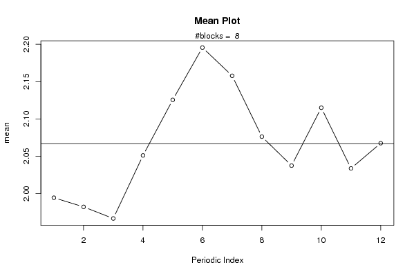
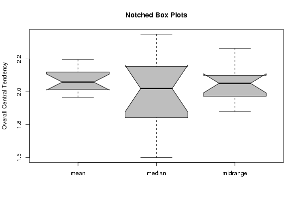
| R Software Module | rwasp_meanplot.wasp | ||||||||||||||||||||
| Title produced by software | Mean Plot | ||||||||||||||||||||
| Date of computation | Thu, 30 Oct 2008 12:18:37 -0600 | ||||||||||||||||||||
| Cite this page as follows | Statistical Computations at FreeStatistics.org, Office for Research Development and Education, URL https://freestatistics.org/blog/index.php?v=date/2008/Oct/30/t1225390821bms6jp3t6ngf6am.htm/, Retrieved Sun, 19 May 2024 15:58:33 +0000 | ||||||||||||||||||||
| Statistical Computations at FreeStatistics.org, Office for Research Development and Education, URL https://freestatistics.org/blog/index.php?pk=20156, Retrieved Sun, 19 May 2024 15:58:33 +0000 | |||||||||||||||||||||
| QR Codes: | |||||||||||||||||||||
|
| |||||||||||||||||||||
| Original text written by user: | |||||||||||||||||||||
| IsPrivate? | No (this computation is public) | ||||||||||||||||||||
| User-defined keywords | |||||||||||||||||||||
| Estimated Impact | 141 | ||||||||||||||||||||
Tree of Dependent Computations | |||||||||||||||||||||
| Family? (F = Feedback message, R = changed R code, M = changed R Module, P = changed Parameters, D = changed Data) | |||||||||||||||||||||
| F [Mean Plot] [workshop 3] [2007-10-26 12:14:28] [e9ffc5de6f8a7be62f22b142b5b6b1a8] F R PD [Mean Plot] [task 4] [2008-10-30 15:40:08] [cb714085b233acee8e8acd879ea442b6] F D [Mean Plot] [task 5: inflatie ...] [2008-10-30 18:18:37] [787873b6436f665b5b192a0bdb2e43c9] [Current] F R PD [Mean Plot] [WS3A T5 pt2] [2008-11-03 21:18:59] [2bdcdcd86f586cbd821f1fe8acabf575] F R PD [Mean Plot] [WS3A T5 pt1] [2008-11-03 21:21:33] [2bdcdcd86f586cbd821f1fe8acabf575] | |||||||||||||||||||||
| Feedback Forum | |||||||||||||||||||||
Post a new message | |||||||||||||||||||||
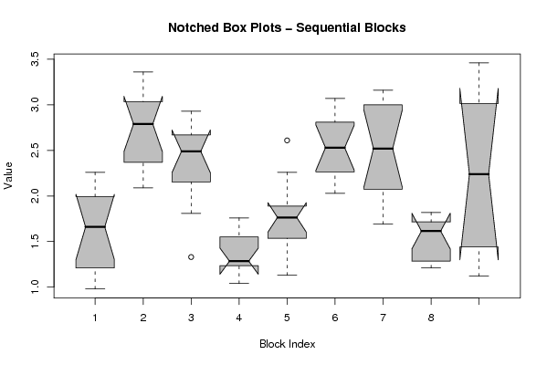
Dataset | |||||||||||||||||||||
| Dataseries X: | |||||||||||||||||||||
0,95 0,98 1,23 1,17 0,84 0,74 0,65 0,91 1,19 1,30 1,53 1,94 1,79 1,95 2,26 2,04 2,16 2,75 2,79 2,88 3,36 2,97 3,10 2,49 2,20 2,25 2,09 2,79 3,14 2,93 2,65 2,67 2,26 2,35 2,13 2,18 2,90 2,63 2,67 1,81 1,33 0,88 1,28 1,26 1,26 1,29 1,10 1,37 1.21 1.74 1.76 1.48 1.04 1.62 1.49 1.79 1.8 1.58 1.86 1.74 1.59 1.26 1.13 1.92 2.61 2.26 2.41 2.26 2.03 2.86 2.55 2.27 2.26 2.57 3.07 2.76 2.51 2.87 3.14 3.11 3.16 2.47 2.57 2.89 2.63 2.38 1.69 1.96 2.19 1.87 1.6 1.63 1.22 1.21 1.49 1.64 1.66 1.77 1.82 1.78 1.28 1.29 1.37 1.12 1.51 2.24 2.94 3.09 3,46 3,64 4,39 4,15 5,21 5,80 5,91 | |||||||||||||||||||||
Tables (Output of Computation) | |||||||||||||||||||||
| |||||||||||||||||||||
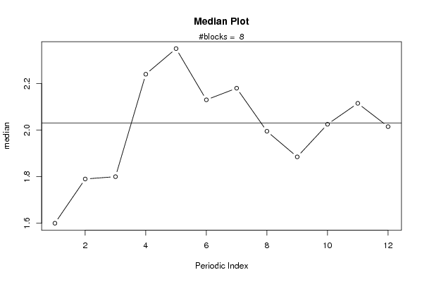
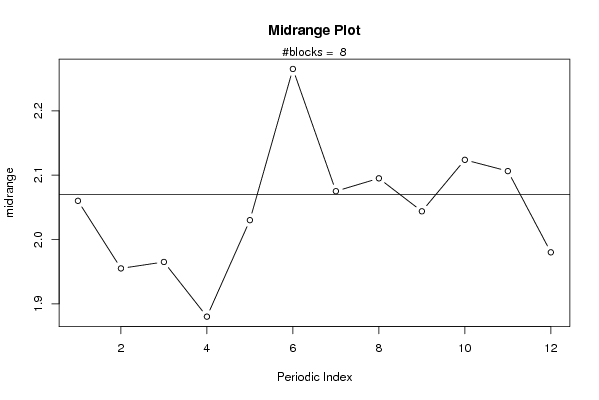
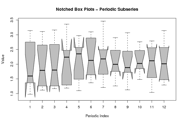
Figures (Output of Computation) | |||||||||||||||||||||
Input Parameters & R Code | |||||||||||||||||||||
| Parameters (Session): | |||||||||||||||||||||
| par1 = grey ; | |||||||||||||||||||||
| Parameters (R input): | |||||||||||||||||||||
| par1 = 12 ; | |||||||||||||||||||||
| R code (references can be found in the software module): | |||||||||||||||||||||
par1 <- as.numeric(par1) | |||||||||||||||||||||