Free Statistics
of Irreproducible Research!
Description of Statistical Computation | |||||||||||||||||||||
|---|---|---|---|---|---|---|---|---|---|---|---|---|---|---|---|---|---|---|---|---|---|
| Author's title | |||||||||||||||||||||
| Author | *The author of this computation has been verified* | ||||||||||||||||||||
| R Software Module | rwasp_meanplot.wasp | ||||||||||||||||||||
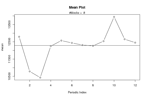
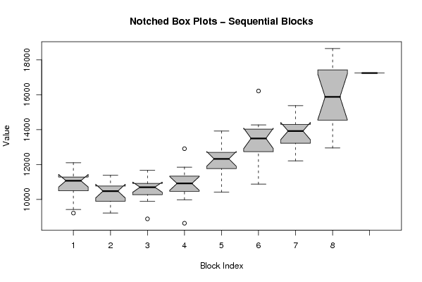
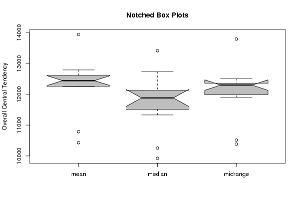
| Title produced by software | Mean Plot | ||||||||||||||||||||
| Date of computation | Thu, 30 Oct 2008 11:45:21 -0600 | ||||||||||||||||||||
| Cite this page as follows | Statistical Computations at FreeStatistics.org, Office for Research Development and Education, URL https://freestatistics.org/blog/index.php?v=date/2008/Oct/30/t12253887551y6qjntfigcjmoi.htm/, Retrieved Sun, 13 Jul 2025 08:04:00 +0000 | ||||||||||||||||||||
| Statistical Computations at FreeStatistics.org, Office for Research Development and Education, URL https://freestatistics.org/blog/index.php?pk=20141, Retrieved Sun, 13 Jul 2025 08:04:00 +0000 | |||||||||||||||||||||
| QR Codes: | |||||||||||||||||||||
|
| |||||||||||||||||||||
| Original text written by user: | |||||||||||||||||||||
| IsPrivate? | No (this computation is public) | ||||||||||||||||||||
| User-defined keywords | |||||||||||||||||||||
| Estimated Impact | 258 | ||||||||||||||||||||
Tree of Dependent Computations | |||||||||||||||||||||
| Family? (F = Feedback message, R = changed R code, M = changed R Module, P = changed Parameters, D = changed Data) | |||||||||||||||||||||
| F [Mean Plot] [workshop 3] [2007-10-26 12:14:28] [e9ffc5de6f8a7be62f22b142b5b6b1a8] F D [Mean Plot] [Q2:Mean plot] [2008-10-30 13:08:02] [1ce0d16c8f4225c977b42c8fa93bc163] F D [Mean Plot] [Task 5(3)] [2008-10-30 17:45:21] [8758b22b4a10c08c31202f233362e983] [Current] | |||||||||||||||||||||
| Feedback Forum | |||||||||||||||||||||
Post a new message | |||||||||||||||||||||
Dataset | |||||||||||||||||||||
| Dataseries X: | |||||||||||||||||||||
10230,4 9221 9428,6 10934,5 10986 11724,6 11180,9 11163,2 11240,9 12107,1 10762,3 11340,4 11266,8 9542,7 9227,7 10571,9 10774,4 10392,8 9920,2 9884,9 10174,5 11395,4 10760,2 10570,1 10536 9902,6 8889 10837,3 11624,1 10509 10984,9 10649,1 10855,7 11677,4 10760,2 10046,2 10772,8 9987,7 8638,7 11063,7 11855,7 10684,5 11337,4 10478 11123,9 12909,3 11339,9 10462,2 12733,5 10519,2 10414,9 12476,8 12384,6 12266,7 12919,9 11497,3 12142 13919,4 12656,8 12034,1 13199,7 10881,3 11301,2 13643,9 12517 13981,1 14275,7 13435 13565,7 16216,3 12970 14079,9 14235 12213,4 12581 14130,4 14210,8 14378,5 13142,8 13714,7 13621,9 15379,8 13306,3 14391,2 14909,9 14025,4 12951,2 14344,3 16213,3 15544,5 14750,6 17292,7 17568,5 17930,8 18644,7 16694,8 17242,8 | |||||||||||||||||||||
Tables (Output of Computation) | |||||||||||||||||||||
| |||||||||||||||||||||
Figures (Output of Computation) | |||||||||||||||||||||
Input Parameters & R Code | |||||||||||||||||||||
| Parameters (Session): | |||||||||||||||||||||
| par1 = 12 ; | |||||||||||||||||||||
| Parameters (R input): | |||||||||||||||||||||
| par1 = 12 ; | |||||||||||||||||||||
| R code (references can be found in the software module): | |||||||||||||||||||||
par1 <- as.numeric(par1) | |||||||||||||||||||||