Free Statistics
of Irreproducible Research!
Description of Statistical Computation | |||||||||||||||||||||
|---|---|---|---|---|---|---|---|---|---|---|---|---|---|---|---|---|---|---|---|---|---|
| Author's title | Mean Plot Buitenlandse handel van Belgi� volgens het nationale concept (maa... | ||||||||||||||||||||
| Author | *The author of this computation has been verified* | ||||||||||||||||||||
| R Software Module | rwasp_meanplot.wasp | ||||||||||||||||||||
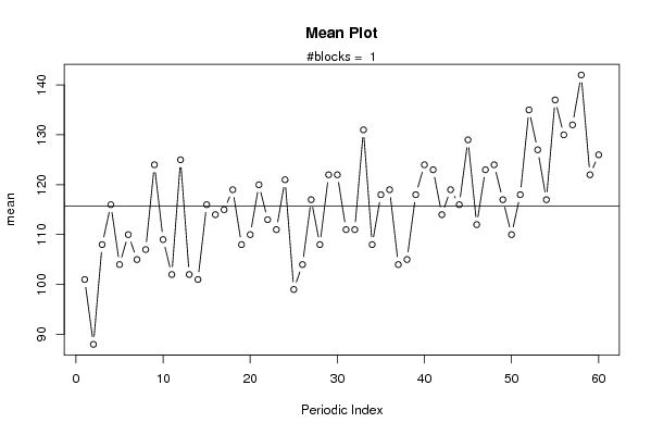
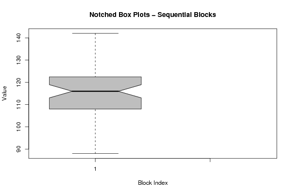
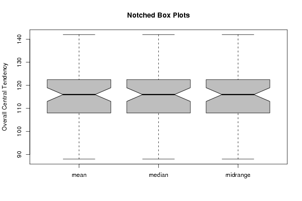
| Title produced by software | Mean Plot | ||||||||||||||||||||
| Date of computation | Thu, 30 Oct 2008 10:16:55 -0600 | ||||||||||||||||||||
| Cite this page as follows | Statistical Computations at FreeStatistics.org, Office for Research Development and Education, URL https://freestatistics.org/blog/index.php?v=date/2008/Oct/30/t1225383463qgpmptu0x2z6rr3.htm/, Retrieved Sun, 19 May 2024 15:26:33 +0000 | ||||||||||||||||||||
| Statistical Computations at FreeStatistics.org, Office for Research Development and Education, URL https://freestatistics.org/blog/index.php?pk=20118, Retrieved Sun, 19 May 2024 15:26:33 +0000 | |||||||||||||||||||||
| QR Codes: | |||||||||||||||||||||
|
| |||||||||||||||||||||
| Original text written by user: | |||||||||||||||||||||
| IsPrivate? | No (this computation is public) | ||||||||||||||||||||
| User-defined keywords | |||||||||||||||||||||
| Estimated Impact | 138 | ||||||||||||||||||||
Tree of Dependent Computations | |||||||||||||||||||||
| Family? (F = Feedback message, R = changed R code, M = changed R Module, P = changed Parameters, D = changed Data) | |||||||||||||||||||||
| F [Univariate Data Series] [Tijdreeks 4 Buite...] [2008-10-13 09:40:00] [58bf45a666dc5198906262e8815a9722] - PD [Univariate Data Series] [Tijdreeks 4 Buite...] [2008-10-20 17:36:31] [58bf45a666dc5198906262e8815a9722] F RMP [Mean Plot] [Mean Plot Buitenl...] [2008-10-30 16:16:55] [63db34dadd44fb018112addcdefe949f] [Current] - P [Mean Plot] [verbetering task ...] [2008-11-07 16:21:45] [3754dd41128068acfc463ebbabce5a9c] | |||||||||||||||||||||
| Feedback Forum | |||||||||||||||||||||
Post a new message | |||||||||||||||||||||
Dataset | |||||||||||||||||||||
| Dataseries X: | |||||||||||||||||||||
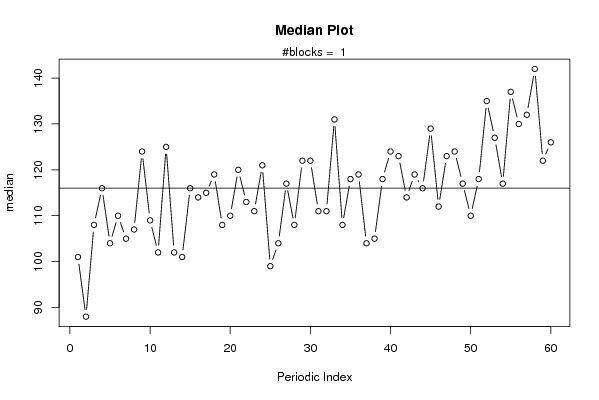
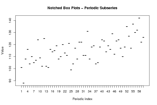
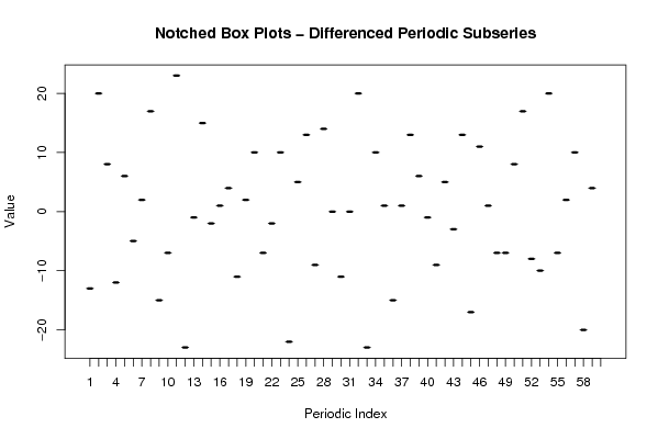
101 88 108 116 104 110 105 107 124 109 102 125 102 101 116 114 115 119 108 110 120 113 111 121 99 104 117 108 122 122 111 111 131 108 118 119 104 105 118 124 123 114 119 116 129 112 123 124 117 110 118 135 127 117 137 130 132 142 122 126 | |||||||||||||||||||||
Tables (Output of Computation) | |||||||||||||||||||||
| |||||||||||||||||||||
Figures (Output of Computation) | |||||||||||||||||||||
Input Parameters & R Code | |||||||||||||||||||||
| Parameters (Session): | |||||||||||||||||||||
| par1 = 60 ; | |||||||||||||||||||||
| Parameters (R input): | |||||||||||||||||||||
| par1 = 60 ; | |||||||||||||||||||||
| R code (references can be found in the software module): | |||||||||||||||||||||
par1 <- as.numeric(par1) | |||||||||||||||||||||