Free Statistics
of Irreproducible Research!
Description of Statistical Computation | |||||||||||||||||||||||||||||||||||||||||||||||||||||||||||||||||||||||||||||||||
|---|---|---|---|---|---|---|---|---|---|---|---|---|---|---|---|---|---|---|---|---|---|---|---|---|---|---|---|---|---|---|---|---|---|---|---|---|---|---|---|---|---|---|---|---|---|---|---|---|---|---|---|---|---|---|---|---|---|---|---|---|---|---|---|---|---|---|---|---|---|---|---|---|---|---|---|---|---|---|---|---|---|
| Author's title | |||||||||||||||||||||||||||||||||||||||||||||||||||||||||||||||||||||||||||||||||
| Author | *The author of this computation has been verified* | ||||||||||||||||||||||||||||||||||||||||||||||||||||||||||||||||||||||||||||||||
| R Software Module | rwasp_bootstrapplot.wasp | ||||||||||||||||||||||||||||||||||||||||||||||||||||||||||||||||||||||||||||||||
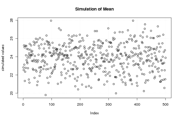
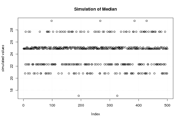
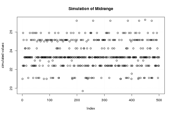
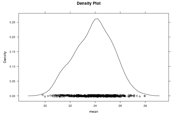
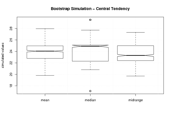
| Title produced by software | Blocked Bootstrap Plot - Central Tendency | ||||||||||||||||||||||||||||||||||||||||||||||||||||||||||||||||||||||||||||||||
| Date of computation | Thu, 30 Oct 2008 07:01:20 -0600 | ||||||||||||||||||||||||||||||||||||||||||||||||||||||||||||||||||||||||||||||||
| Cite this page as follows | Statistical Computations at FreeStatistics.org, Office for Research Development and Education, URL https://freestatistics.org/blog/index.php?v=date/2008/Oct/30/t1225371981poch1yy00txtlce.htm/, Retrieved Sat, 05 Jul 2025 19:54:19 +0000 | ||||||||||||||||||||||||||||||||||||||||||||||||||||||||||||||||||||||||||||||||
| Statistical Computations at FreeStatistics.org, Office for Research Development and Education, URL https://freestatistics.org/blog/index.php?pk=20001, Retrieved Sat, 05 Jul 2025 19:54:19 +0000 | |||||||||||||||||||||||||||||||||||||||||||||||||||||||||||||||||||||||||||||||||
| QR Codes: | |||||||||||||||||||||||||||||||||||||||||||||||||||||||||||||||||||||||||||||||||
|
| |||||||||||||||||||||||||||||||||||||||||||||||||||||||||||||||||||||||||||||||||
| Original text written by user: | |||||||||||||||||||||||||||||||||||||||||||||||||||||||||||||||||||||||||||||||||
| IsPrivate? | No (this computation is public) | ||||||||||||||||||||||||||||||||||||||||||||||||||||||||||||||||||||||||||||||||
| User-defined keywords | |||||||||||||||||||||||||||||||||||||||||||||||||||||||||||||||||||||||||||||||||
| Estimated Impact | 268 | ||||||||||||||||||||||||||||||||||||||||||||||||||||||||||||||||||||||||||||||||
Tree of Dependent Computations | |||||||||||||||||||||||||||||||||||||||||||||||||||||||||||||||||||||||||||||||||
| Family? (F = Feedback message, R = changed R code, M = changed R Module, P = changed Parameters, D = changed Data) | |||||||||||||||||||||||||||||||||||||||||||||||||||||||||||||||||||||||||||||||||
| - [Blocked Bootstrap Plot - Central Tendency] [Taak 5 deel 2 Q1 ...] [2008-10-30 13:01:20] [286e96bd53289970f8e5f25a93fb50b3] [Current] - RM D [Pearson Correlation] [Taak 5 deel 2 Q1 ...] [2008-10-30 13:33:26] [819b576fab25b35cfda70f80599828ec] - RM D [Pearson Correlation] [Taak 5 deel 2 Q1 ...] [2008-10-30 13:39:26] [819b576fab25b35cfda70f80599828ec] - RM D [Pearson Correlation] [Taak 5 deel 2 Q1 ...] [2008-10-30 13:42:36] [6fea0e9a9b3b29a63badf2c274e82506] - RM D [Pearson Correlation] [Taak 5 deel 2 Q1 ...] [2008-10-30 13:45:27] [6fea0e9a9b3b29a63badf2c274e82506] F RM D [Star Plot] [Task 5 Deel 2 Q2 ...] [2008-10-30 14:15:09] [819b576fab25b35cfda70f80599828ec] F RM D [Mean Plot] [Taak 5 deel 2 Q3 ...] [2008-10-30 14:47:33] [6fea0e9a9b3b29a63badf2c274e82506] - RM D [Mean Plot] [Taak 5 deel 2 Q3 ...] [2008-10-30 15:05:13] [819b576fab25b35cfda70f80599828ec] - RM D [Mean Plot] [Taak 5 deel 2 Q3 ...] [2008-10-30 15:10:04] [819b576fab25b35cfda70f80599828ec] - RM D [Mean Plot] [Taak 5 deel 2 Q3 ...] [2008-10-30 15:12:54] [6fea0e9a9b3b29a63badf2c274e82506] - RM D [Mean Plot] [Taak 5 deel 2 Q3 ...] [2008-10-30 15:15:09] [819b576fab25b35cfda70f80599828ec] F RM D [Notched Boxplots] [Taak 5 deel 1 tas...] [2008-10-30 15:39:12] [6fea0e9a9b3b29a63badf2c274e82506] F R PD [Notched Boxplots] [Taak 5 Deel 1 Task 3] [2008-11-03 16:24:11] [6fea0e9a9b3b29a63badf2c274e82506] | |||||||||||||||||||||||||||||||||||||||||||||||||||||||||||||||||||||||||||||||||
| Feedback Forum | |||||||||||||||||||||||||||||||||||||||||||||||||||||||||||||||||||||||||||||||||
Post a new message | |||||||||||||||||||||||||||||||||||||||||||||||||||||||||||||||||||||||||||||||||
Dataset | |||||||||||||||||||||||||||||||||||||||||||||||||||||||||||||||||||||||||||||||||
| Dataseries X: | |||||||||||||||||||||||||||||||||||||||||||||||||||||||||||||||||||||||||||||||||
20,8 17,1 22,3 25,1 27,7 24,9 29,5 | |||||||||||||||||||||||||||||||||||||||||||||||||||||||||||||||||||||||||||||||||
Tables (Output of Computation) | |||||||||||||||||||||||||||||||||||||||||||||||||||||||||||||||||||||||||||||||||
| |||||||||||||||||||||||||||||||||||||||||||||||||||||||||||||||||||||||||||||||||
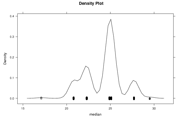
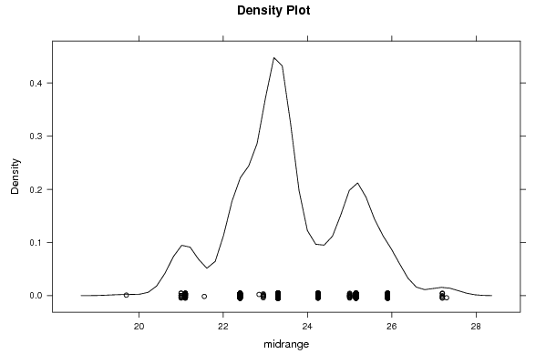
Figures (Output of Computation) | |||||||||||||||||||||||||||||||||||||||||||||||||||||||||||||||||||||||||||||||||
Input Parameters & R Code | |||||||||||||||||||||||||||||||||||||||||||||||||||||||||||||||||||||||||||||||||
| Parameters (Session): | |||||||||||||||||||||||||||||||||||||||||||||||||||||||||||||||||||||||||||||||||
| par1 = 500 ; par2 = 12 ; | |||||||||||||||||||||||||||||||||||||||||||||||||||||||||||||||||||||||||||||||||
| Parameters (R input): | |||||||||||||||||||||||||||||||||||||||||||||||||||||||||||||||||||||||||||||||||
| par1 = 500 ; par2 = 12 ; | |||||||||||||||||||||||||||||||||||||||||||||||||||||||||||||||||||||||||||||||||
| R code (references can be found in the software module): | |||||||||||||||||||||||||||||||||||||||||||||||||||||||||||||||||||||||||||||||||
par1 <- as.numeric(par1) | |||||||||||||||||||||||||||||||||||||||||||||||||||||||||||||||||||||||||||||||||