Free Statistics
of Irreproducible Research!
Description of Statistical Computation | |||||||||||||||||||||
|---|---|---|---|---|---|---|---|---|---|---|---|---|---|---|---|---|---|---|---|---|---|
| Author's title | |||||||||||||||||||||
| Author | *The author of this computation has been verified* | ||||||||||||||||||||
| R Software Module | rwasp_meanplot.wasp | ||||||||||||||||||||
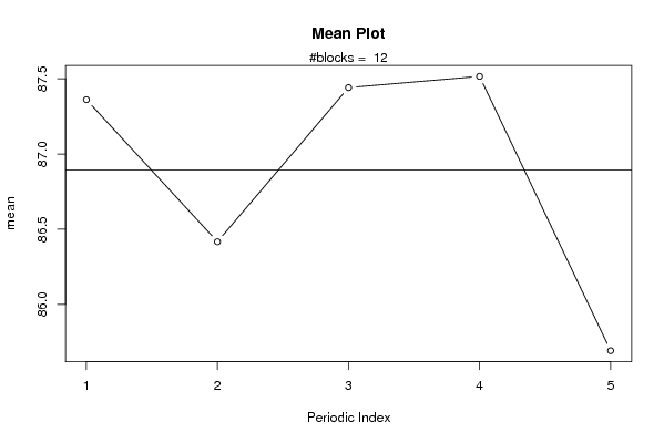
| Title produced by software | Mean Plot | ||||||||||||||||||||
| Date of computation | Thu, 30 Oct 2008 05:54:43 -0600 | ||||||||||||||||||||
| Cite this page as follows | Statistical Computations at FreeStatistics.org, Office for Research Development and Education, URL https://freestatistics.org/blog/index.php?v=date/2008/Oct/30/t122536776325sqo48amn5wm4a.htm/, Retrieved Sun, 19 May 2024 14:08:46 +0000 | ||||||||||||||||||||
| Statistical Computations at FreeStatistics.org, Office for Research Development and Education, URL https://freestatistics.org/blog/index.php?pk=19982, Retrieved Sun, 19 May 2024 14:08:46 +0000 | |||||||||||||||||||||
| QR Codes: | |||||||||||||||||||||
|
| |||||||||||||||||||||
| Original text written by user: | |||||||||||||||||||||
| IsPrivate? | No (this computation is public) | ||||||||||||||||||||
| User-defined keywords | |||||||||||||||||||||
| Estimated Impact | 244 | ||||||||||||||||||||
Tree of Dependent Computations | |||||||||||||||||||||
| Family? (F = Feedback message, R = changed R code, M = changed R Module, P = changed Parameters, D = changed Data) | |||||||||||||||||||||
| F [Mean Plot] [workshop 3] [2007-10-26 12:14:28] [e9ffc5de6f8a7be62f22b142b5b6b1a8] F PD [Mean Plot] [mean plot Q 3] [2008-10-30 11:54:43] [a8228479d4547a92e2d3f176a5299609] [Current] F [Mean Plot] [Q3] [2008-11-03 17:22:30] [4ad596f10399a71ad29b7d76e6ab90ac] - P [Mean Plot] [q3] [2008-11-07 18:29:52] [4ad596f10399a71ad29b7d76e6ab90ac] F [Mean Plot] [Task 1 Q3] [2008-11-03 18:54:10] [005293453b571dbccb80b45226e44173] F P [Mean Plot] [Task 1 Q3] [2008-11-03 18:56:21] [005293453b571dbccb80b45226e44173] F [Mean Plot] [] [2008-11-03 20:42:04] [af90f76a5211a482a7c35f2c76d2fd61] F [Mean Plot] [] [2008-11-03 20:44:59] [af90f76a5211a482a7c35f2c76d2fd61] F [Mean Plot] [] [2008-11-03 21:05:14] [29747f79f5beb5b2516e1271770ecb47] F [Mean Plot] [] [2008-11-03 21:06:18] [29747f79f5beb5b2516e1271770ecb47] - P [Mean Plot] [Q3] [2008-11-05 18:33:05] [ed2ba3b6182103c15c0ab511ae4e6284] - [Mean Plot] [verbetering Q3] [2008-11-07 16:53:17] [2bd2ad6af3eef3a703e9ec23e39bd695] | |||||||||||||||||||||
| Feedback Forum | |||||||||||||||||||||
Post a new message | |||||||||||||||||||||
Dataset | |||||||||||||||||||||
| Dataseries X: | |||||||||||||||||||||
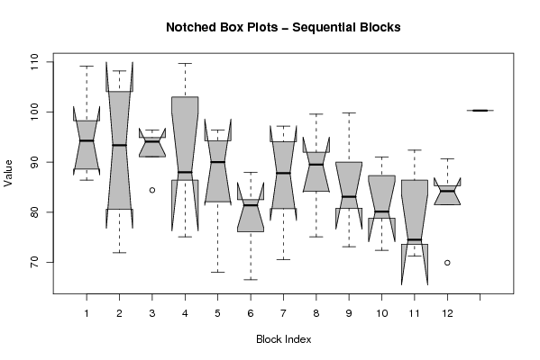
109.20 88.60 94.30 98.30 86.40 80.60 104.10 108.20 93.40 71.90 94.10 94.90 96.40 91.10 84.40 86.40 88.00 75.10 109.70 103.00 82.10 68.00 96.40 94.30 90.00 88.00 76.10 82.50 81.40 66.50 97.20 94.10 80.70 70.50 87.80 89.50 99.60 84.20 75.10 92.00 80.80 73.10 99.80 90.00 83.10 72.40 78.80 87.30 91.00 80.10 73.60 86.40 74.50 71.20 92.40 81.50 85.30 69.90 84.20 90.70 100.30 | |||||||||||||||||||||
Tables (Output of Computation) | |||||||||||||||||||||
| |||||||||||||||||||||
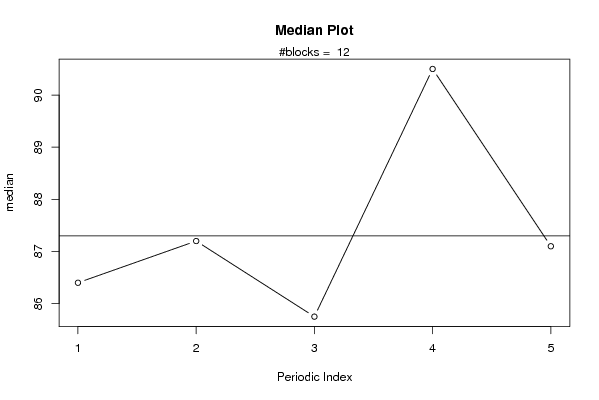
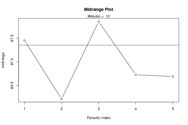
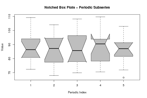
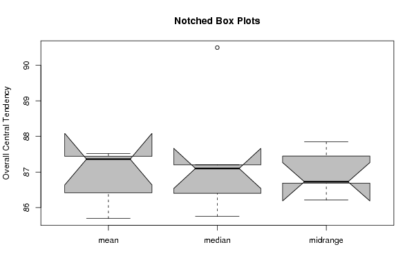
Figures (Output of Computation) | |||||||||||||||||||||
Input Parameters & R Code | |||||||||||||||||||||
| Parameters (Session): | |||||||||||||||||||||
| par1 = 5 ; | |||||||||||||||||||||
| Parameters (R input): | |||||||||||||||||||||
| par1 = 5 ; | |||||||||||||||||||||
| R code (references can be found in the software module): | |||||||||||||||||||||
par1 <- as.numeric(par1) | |||||||||||||||||||||