Free Statistics
of Irreproducible Research!
Description of Statistical Computation | |||||||||||||||||||||||||||||||||||||||||||||||||||||
|---|---|---|---|---|---|---|---|---|---|---|---|---|---|---|---|---|---|---|---|---|---|---|---|---|---|---|---|---|---|---|---|---|---|---|---|---|---|---|---|---|---|---|---|---|---|---|---|---|---|---|---|---|---|
| Author's title | |||||||||||||||||||||||||||||||||||||||||||||||||||||
| Author | *The author of this computation has been verified* | ||||||||||||||||||||||||||||||||||||||||||||||||||||
| R Software Module | rwasp_edauni.wasp | ||||||||||||||||||||||||||||||||||||||||||||||||||||
| Title produced by software | Univariate Explorative Data Analysis | ||||||||||||||||||||||||||||||||||||||||||||||||||||
| Date of computation | Tue, 28 Oct 2008 09:31:05 -0600 | ||||||||||||||||||||||||||||||||||||||||||||||||||||
| Cite this page as follows | Statistical Computations at FreeStatistics.org, Office for Research Development and Education, URL https://freestatistics.org/blog/index.php?v=date/2008/Oct/28/t1225207976qfcmnln0xwqllwn.htm/, Retrieved Wed, 02 Jul 2025 02:57:51 +0000 | ||||||||||||||||||||||||||||||||||||||||||||||||||||
| Statistical Computations at FreeStatistics.org, Office for Research Development and Education, URL https://freestatistics.org/blog/index.php?pk=19776, Retrieved Wed, 02 Jul 2025 02:57:51 +0000 | |||||||||||||||||||||||||||||||||||||||||||||||||||||
| QR Codes: | |||||||||||||||||||||||||||||||||||||||||||||||||||||
|
| |||||||||||||||||||||||||||||||||||||||||||||||||||||
| Original text written by user: | |||||||||||||||||||||||||||||||||||||||||||||||||||||
| IsPrivate? | No (this computation is public) | ||||||||||||||||||||||||||||||||||||||||||||||||||||
| User-defined keywords | |||||||||||||||||||||||||||||||||||||||||||||||||||||
| Estimated Impact | 306 | ||||||||||||||||||||||||||||||||||||||||||||||||||||
Tree of Dependent Computations | |||||||||||||||||||||||||||||||||||||||||||||||||||||
| Family? (F = Feedback message, R = changed R code, M = changed R Module, P = changed Parameters, D = changed Data) | |||||||||||||||||||||||||||||||||||||||||||||||||||||
| F [Univariate Data Series] [Prijsindexcijfer ...] [2008-10-13 23:09:34] [2f3410588adf1243d1e1cac6ff48a9c9] - PD [Univariate Data Series] [Bouwproductie] [2008-10-28 07:22:13] [f5709eefd05c649ca6dad46019ffd879] - PD [Univariate Data Series] [Bouwvergunningen] [2008-10-28 07:26:05] [f5709eefd05c649ca6dad46019ffd879] - PD [Univariate Data Series] [Werkloosheid] [2008-10-28 07:28:46] [f5709eefd05c649ca6dad46019ffd879] F RMPD [Univariate Explorative Data Analysis] [Kledingproductie] [2008-10-28 07:43:38] [f5709eefd05c649ca6dad46019ffd879] - PD [Univariate Explorative Data Analysis] [Productie Kleding] [2008-10-28 15:31:05] [28deb8481dba3cc87d2d53a86e0e0d0b] [Current] - RMP [Central Tendency] [kleding productie...] [2008-10-28 15:58:15] [f5709eefd05c649ca6dad46019ffd879] F D [Univariate Explorative Data Analysis] [kledingproductie/...] [2008-10-28 16:22:17] [f5709eefd05c649ca6dad46019ffd879] - RMP [Harrell-Davis Quantiles] [q3 harrel davis] [2008-10-28 16:41:47] [f5709eefd05c649ca6dad46019ffd879] - RMP [Central Tendency] [central tendency,...] [2008-10-29 14:00:39] [f5709eefd05c649ca6dad46019ffd879] | |||||||||||||||||||||||||||||||||||||||||||||||||||||
| Feedback Forum | |||||||||||||||||||||||||||||||||||||||||||||||||||||
Post a new message | |||||||||||||||||||||||||||||||||||||||||||||||||||||
Dataset | |||||||||||||||||||||||||||||||||||||||||||||||||||||
| Dataseries X: | |||||||||||||||||||||||||||||||||||||||||||||||||||||
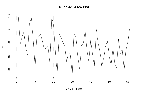
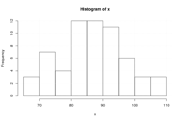
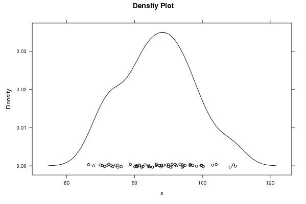
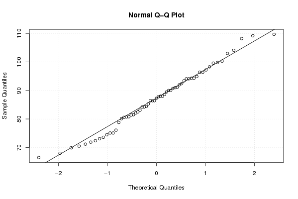
109.20 88.60 94.30 98.30 86.40 80.60 104.10 108.20 93.40 71.90 94.10 94.90 96.40 91.10 84.40 86.40 88.00 75.10 109.70 103.00 82.10 68.00 96.40 94.30 90.00 88.00 76.10 82.50 81.40 66.50 97.20 94.10 80.70 70.50 87.80 89.50 99.60 84.20 75.10 92.00 80.80 73.10 99.80 90.00 83.10 72.40 78.80 87.30 91.00 80.10 73.60 86.40 74.50 71.20 92.40 81.50 85.30 69.90 84.20 90.70 100.30 | |||||||||||||||||||||||||||||||||||||||||||||||||||||
Tables (Output of Computation) | |||||||||||||||||||||||||||||||||||||||||||||||||||||
| |||||||||||||||||||||||||||||||||||||||||||||||||||||
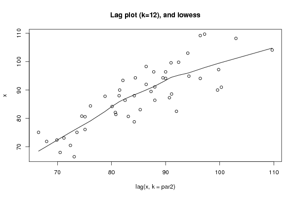
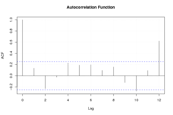
Figures (Output of Computation) | |||||||||||||||||||||||||||||||||||||||||||||||||||||
Input Parameters & R Code | |||||||||||||||||||||||||||||||||||||||||||||||||||||
| Parameters (Session): | |||||||||||||||||||||||||||||||||||||||||||||||||||||
| par1 = 0 ; par2 = 12 ; | |||||||||||||||||||||||||||||||||||||||||||||||||||||
| Parameters (R input): | |||||||||||||||||||||||||||||||||||||||||||||||||||||
| par1 = 0 ; par2 = 12 ; | |||||||||||||||||||||||||||||||||||||||||||||||||||||
| R code (references can be found in the software module): | |||||||||||||||||||||||||||||||||||||||||||||||||||||
par1 <- as.numeric(par1) | |||||||||||||||||||||||||||||||||||||||||||||||||||||