Repository of Reproducible Computations

Free Statistics

of Irreproducible Research!

Author's title

Author

*The author of this computation has been verified*

R Software Module

rwasp_edauni.wasp

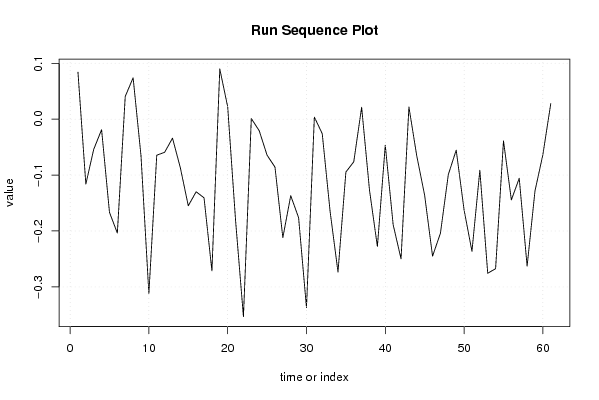
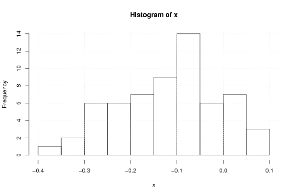
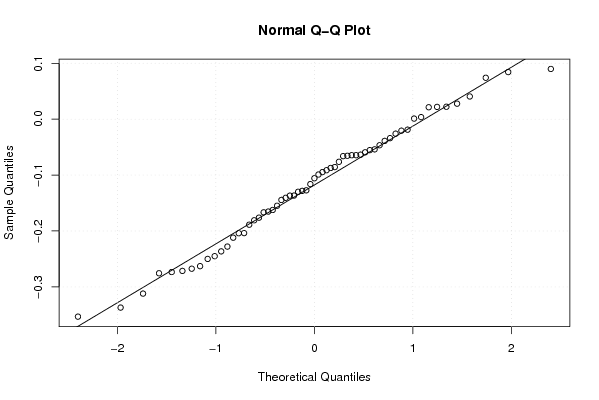
Title produced by software

Univariate Explorative Data Analysis

Date of computation

Mon, 27 Oct 2008 16:19:22 -0600

Cite this page as follows

Statistical Computations at FreeStatistics.org, Office for Research Development and Education, URL https://freestatistics.org/blog/index.php?v=date/2008/Oct/27/t1225146004v08vn8g9nbyu6a1.htm/, Retrieved Sun, 19 May 2024 15:24:29 +0000

Statistical Computations at FreeStatistics.org, Office for Research Development and Education, URL https://freestatistics.org/blog/index.php?pk=19689, Retrieved Sun, 19 May 2024 15:24:29 +0000

QR Codes:

Paste this QR Code to cite your computation.

Original text written by user:

IsPrivate?

No (this computation is public)

User-defined keywords

Estimated Impact

125

Family? (F = Feedback message, R = changed R code, M = changed R Module, P = changed Parameters, D = changed Data)

F     [Univariate Explorative Data Analysis] [Investigation val...] [2008-10-26 16:57:19] [2d9298e0f43790a501ecec52b0f4048b]
-         [Univariate Explorative Data Analysis] [Investigating Values] [2008-10-27 22:19:22] [07b7cf1321bc38017c2c7efcf91ca696] [Current]

Feedback Forum

Post a new message

Dataseries X:

Download CSV

Histogram

Boxplots

0,08423913
-0,116182573
-0,053974485
-0,018832392
-0,166666667
-0,203801478
0,040594059
0,074040219
-0,065493646
-0,312017641
-0,064449064
-0,059313215
-0,033962264
-0,087293889
-0,154901961
-0,129894938
-0,140697674
-0,271444083
0,089803555
0,022202487
-0,180924287
-0,35326087
0,001026694
-0,020618557
-0,064516129
-0,085686465
-0,212028542
-0,136842105
-0,176201373
-0,337041157
0,003642987
-0,025962399
-0,165314402
-0,273477812
-0,094637224
-0,07628866
0,021295475
-0,127308066
-0,227926078
-0,046678636
-0,188787185
-0,25
0,021910605
-0,066183137
-0,136669875
-0,24507874
-0,204016913
-0,099061522
-0,055396371
-0,162451362
-0,236493374
-0,091308165
-0,275648949
-0,267502612
-0,038869258
-0,144475921
-0,105698529
-0,262952102
-0,128282828
-0,063555114
0,027705628

Summary of computational transaction
Raw Input	view raw input (R code)
Raw Output	view raw output of R engine
Computing time	2 seconds
R Server	'George Udny Yule' @ 72.249.76.132

\begin{tabular}{lllllllll}
\hline
Summary of computational transaction \tabularnewline
Raw Input & view raw input (R code)  \tabularnewline
Raw Output & view raw output of R engine  \tabularnewline
Computing time & 2 seconds \tabularnewline
R Server & 'George Udny Yule' @ 72.249.76.132 \tabularnewline
\hline
\end{tabular}
%Source: https://freestatistics.org/blog/index.php?pk=19689&T=0

[TABLE]
[ROW][C]Summary of computational transaction[/C][/ROW]
[ROW][C]Raw Input[/C][C]view raw input (R code) [/C][/ROW]
[ROW][C]Raw Output[/C][C]view raw output of R engine [/C][/ROW]
[ROW][C]Computing time[/C][C]2 seconds[/C][/ROW]
[ROW][C]R Server[/C][C]'George Udny Yule' @ 72.249.76.132[/C][/ROW]
[/TABLE]
Source: https://freestatistics.org/blog/index.php?pk=19689&T=0

Globally Unique Identifier (entire table): ba.freestatistics.org/blog/index.php?pk=19689&T=0

As an alternative you can also use a QR Code:

The GUIDs for individual cells are displayed in the table below:

Summary of computational transaction
Raw Input	view raw input (R code)
Raw Output	view raw output of R engine
Computing time	2 seconds
R Server	'George Udny Yule' @ 72.249.76.132

Descriptive Statistics
# observations	61
minimum	-0.35326087
Q1	-0.188787185
median	-0.105698529
mean	-0.116714915573770
Q3	-0.046678636
maximum	0.089803555

\begin{tabular}{lllllllll}
\hline
Descriptive Statistics \tabularnewline
# observations & 61 \tabularnewline
minimum & -0.35326087 \tabularnewline
Q1 & -0.188787185 \tabularnewline
median & -0.105698529 \tabularnewline
mean & -0.116714915573770 \tabularnewline
Q3 & -0.046678636 \tabularnewline
maximum & 0.089803555 \tabularnewline
\hline
\end{tabular}
%Source: https://freestatistics.org/blog/index.php?pk=19689&T=1

[TABLE]
[ROW][C]Descriptive Statistics[/C][/ROW]
[ROW][C]# observations[/C][C]61[/C][/ROW]
[ROW][C]minimum[/C][C]-0.35326087[/C][/ROW]
[ROW][C]Q1[/C][C]-0.188787185[/C][/ROW]
[ROW][C]median[/C][C]-0.105698529[/C][/ROW]
[ROW][C]mean[/C][C]-0.116714915573770[/C][/ROW]
[ROW][C]Q3[/C][C]-0.046678636[/C][/ROW]
[ROW][C]maximum[/C][C]0.089803555[/C][/ROW]
[/TABLE]
Source: https://freestatistics.org/blog/index.php?pk=19689&T=1

Globally Unique Identifier (entire table): ba.freestatistics.org/blog/index.php?pk=19689&T=1

As an alternative you can also use a QR Code:

The GUIDs for individual cells are displayed in the table below:

Descriptive Statistics
# observations	61
minimum	-0.35326087
Q1	-0.188787185
median	-0.105698529
mean	-0.116714915573770
Q3	-0.046678636
maximum	0.089803555

Figure 1

PNG link

Postscript link

PDF link

Figure 2

PNG link

Postscript link

PDF link

Figure 3

PNG link

Postscript link

PDF link

Figure 4

PNG link

Postscript link

PDF link

Figure 5

PNG link

Postscript link

PDF link

Figure 6

PNG link

Postscript link

PDF link

Figure 7

PNG link

Postscript link

PDF link

Parameters (Session):

par1 = 0 ; par2 = 0 ;

Parameters (R input):

par1 = 0 ; par2 = 0 ; par3 = ; par4 = ; par5 = ; par6 = ; par7 = ; par8 = ; par9 = ; par10 = ; par11 = ; par12 = ; par13 = ; par14 = ; par15 = ; par16 = ; par17 = ; par18 = ; par19 = ; par20 = ;

R code (references can be found in the software module):

par1 <- as.numeric(par1)
par2 <- as.numeric(par2)
x <- as.ts(x)
library(lattice)
bitmap(file='pic1.png')
plot(x,type='l',main='Run Sequence Plot',xlab='time or index',ylab='value')
grid()
dev.off()
bitmap(file='pic2.png')
hist(x)
grid()
dev.off()
bitmap(file='pic3.png')
if (par1 > 0)
{
densityplot(~x,col='black',main=paste('Density Plot   bw = ',par1),bw=par1)
} else {
densityplot(~x,col='black',main='Density Plot')
}
dev.off()
bitmap(file='pic4.png')
qqnorm(x)
qqline(x)
grid()
dev.off()
if (par2 > 0)
{
bitmap(file='lagplot1.png')
dum <- cbind(lag(x,k=1),x)
dum
dum1 <- dum[2:length(x),]
dum1
z <- as.data.frame(dum1)
z
plot(z,main='Lag plot (k=1), lowess, and regression line')
lines(lowess(z))
abline(lm(z))
dev.off()
if (par2 > 1) {
bitmap(file='lagplotpar2.png')
dum <- cbind(lag(x,k=par2),x)
dum
dum1 <- dum[(par2+1):length(x),]
dum1
z <- as.data.frame(dum1)
z
mylagtitle <- 'Lag plot (k='
mylagtitle <- paste(mylagtitle,par2,sep='')
mylagtitle <- paste(mylagtitle,'), and lowess',sep='')
plot(z,main=mylagtitle)
lines(lowess(z))
dev.off()
}
bitmap(file='pic5.png')
acf(x,lag.max=par2,main='Autocorrelation Function')
grid()
dev.off()
}
summary(x)
load(file='createtable')
a<-table.start()
a<-table.row.start(a)
a<-table.element(a,'Descriptive Statistics',2,TRUE)
a<-table.row.end(a)
a<-table.row.start(a)
a<-table.element(a,'# observations',header=TRUE)
a<-table.element(a,length(x))
a<-table.row.end(a)
a<-table.row.start(a)
a<-table.element(a,'minimum',header=TRUE)
a<-table.element(a,min(x))
a<-table.row.end(a)
a<-table.row.start(a)
a<-table.element(a,'Q1',header=TRUE)
a<-table.element(a,quantile(x,0.25))
a<-table.row.end(a)
a<-table.row.start(a)
a<-table.element(a,'median',header=TRUE)
a<-table.element(a,median(x))
a<-table.row.end(a)
a<-table.row.start(a)
a<-table.element(a,'mean',header=TRUE)
a<-table.element(a,mean(x))
a<-table.row.end(a)
a<-table.row.start(a)
a<-table.element(a,'Q3',header=TRUE)
a<-table.element(a,quantile(x,0.75))
a<-table.row.end(a)
a<-table.row.start(a)
a<-table.element(a,'maximum',header=TRUE)
a<-table.element(a,max(x))
a<-table.row.end(a)
a<-table.end(a)
table.save(a,file='mytable.tab')

Free Statistics

Description of Statistical Computation

Tree of Dependent Computations

Dataset

Tables (Output of Computation)

Figures (Output of Computation)

Input Parameters & R Code