Free Statistics
of Irreproducible Research!
Description of Statistical Computation | |||||||||||||||||||||||||||||||||||||||||||||||||||||
|---|---|---|---|---|---|---|---|---|---|---|---|---|---|---|---|---|---|---|---|---|---|---|---|---|---|---|---|---|---|---|---|---|---|---|---|---|---|---|---|---|---|---|---|---|---|---|---|---|---|---|---|---|---|
| Author's title | |||||||||||||||||||||||||||||||||||||||||||||||||||||
| Author | *The author of this computation has been verified* | ||||||||||||||||||||||||||||||||||||||||||||||||||||
| R Software Module | rwasp_edauni.wasp | ||||||||||||||||||||||||||||||||||||||||||||||||||||
| Title produced by software | Univariate Explorative Data Analysis | ||||||||||||||||||||||||||||||||||||||||||||||||||||
| Date of computation | Mon, 27 Oct 2008 13:13:58 -0600 | ||||||||||||||||||||||||||||||||||||||||||||||||||||
| Cite this page as follows | Statistical Computations at FreeStatistics.org, Office for Research Development and Education, URL https://freestatistics.org/blog/index.php?v=date/2008/Oct/27/t1225134917oxgdsj5ycfwcjvd.htm/, Retrieved Sun, 19 May 2024 13:35:38 +0000 | ||||||||||||||||||||||||||||||||||||||||||||||||||||
| Statistical Computations at FreeStatistics.org, Office for Research Development and Education, URL https://freestatistics.org/blog/index.php?pk=19435, Retrieved Sun, 19 May 2024 13:35:38 +0000 | |||||||||||||||||||||||||||||||||||||||||||||||||||||
| QR Codes: | |||||||||||||||||||||||||||||||||||||||||||||||||||||
|
| |||||||||||||||||||||||||||||||||||||||||||||||||||||
| Original text written by user: | |||||||||||||||||||||||||||||||||||||||||||||||||||||
| IsPrivate? | No (this computation is public) | ||||||||||||||||||||||||||||||||||||||||||||||||||||
| User-defined keywords | |||||||||||||||||||||||||||||||||||||||||||||||||||||
| Estimated Impact | 135 | ||||||||||||||||||||||||||||||||||||||||||||||||||||
Tree of Dependent Computations | |||||||||||||||||||||||||||||||||||||||||||||||||||||
| Family? (F = Feedback message, R = changed R code, M = changed R Module, P = changed Parameters, D = changed Data) | |||||||||||||||||||||||||||||||||||||||||||||||||||||
| F [Univariate Explorative Data Analysis] [Investigation Dis...] [2007-10-21 17:06:37] [b9964c45117f7aac638ab9056d451faa] F D [Univariate Explorative Data Analysis] [Q2 Univariate exp...] [2008-10-27 18:42:20] [d134696a922d84037f02d49ded84b0bd] F D [Univariate Explorative Data Analysis] [Univariate explor...] [2008-10-27 19:13:58] [db9a5fd0f9c3e1245d8075d8bb09236d] [Current] - D [Univariate Explorative Data Analysis] [Univariate explor...] [2008-10-27 19:16:43] [d134696a922d84037f02d49ded84b0bd] - PD [Univariate Explorative Data Analysis] [Q7] [2008-11-03 18:58:29] [d134696a922d84037f02d49ded84b0bd] | |||||||||||||||||||||||||||||||||||||||||||||||||||||
| Feedback Forum | |||||||||||||||||||||||||||||||||||||||||||||||||||||
Post a new message | |||||||||||||||||||||||||||||||||||||||||||||||||||||
Dataset | |||||||||||||||||||||||||||||||||||||||||||||||||||||
| Dataseries X: | |||||||||||||||||||||||||||||||||||||||||||||||||||||
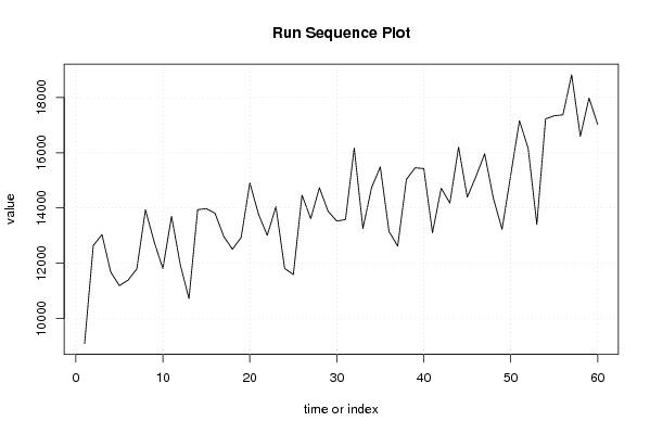
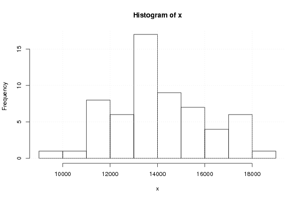
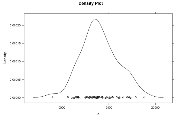
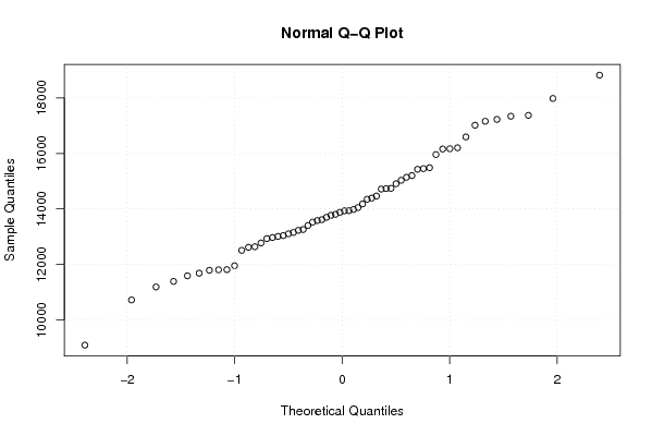
9097,4 12639,8 13040,1 11687,3 11191,7 11391,9 11793,1 13933,2 12778,1 11810,3 13698,4 11956,6 10723,8 13938,9 13979,8 13807,4 12973,9 12509,8 12934,1 14908,3 13772,1 13012,6 14049,9 11816,5 11593,2 14466,2 13615,9 14733,9 13880,7 13527,5 13584 16170,2 13260,6 14741,9 15486,5 13154,5 12621,2 15031,6 15452,4 15428 13105,9 14716,8 14180 16202,2 14392,4 15140,6 15960,1 14351,3 13230,2 15202,1 17157,3 16159,1 13405,7 17224,7 17338,4 17370,6 18817,8 16593,2 17979,5 17015,2 | |||||||||||||||||||||||||||||||||||||||||||||||||||||
Tables (Output of Computation) | |||||||||||||||||||||||||||||||||||||||||||||||||||||
| |||||||||||||||||||||||||||||||||||||||||||||||||||||
Figures (Output of Computation) | |||||||||||||||||||||||||||||||||||||||||||||||||||||
Input Parameters & R Code | |||||||||||||||||||||||||||||||||||||||||||||||||||||
| Parameters (Session): | |||||||||||||||||||||||||||||||||||||||||||||||||||||
| par1 = 0 ; par2 = 0 ; | |||||||||||||||||||||||||||||||||||||||||||||||||||||
| Parameters (R input): | |||||||||||||||||||||||||||||||||||||||||||||||||||||
| par1 = 0 ; par2 = 0 ; | |||||||||||||||||||||||||||||||||||||||||||||||||||||
| R code (references can be found in the software module): | |||||||||||||||||||||||||||||||||||||||||||||||||||||
par1 <- as.numeric(par1) | |||||||||||||||||||||||||||||||||||||||||||||||||||||