Free Statistics
of Irreproducible Research!
Description of Statistical Computation | |||||||||||||||||||||||||||||||||||||||||||||||||||||
|---|---|---|---|---|---|---|---|---|---|---|---|---|---|---|---|---|---|---|---|---|---|---|---|---|---|---|---|---|---|---|---|---|---|---|---|---|---|---|---|---|---|---|---|---|---|---|---|---|---|---|---|---|---|
| Author's title | |||||||||||||||||||||||||||||||||||||||||||||||||||||
| Author | *The author of this computation has been verified* | ||||||||||||||||||||||||||||||||||||||||||||||||||||
| R Software Module | rwasp_edauni.wasp | ||||||||||||||||||||||||||||||||||||||||||||||||||||
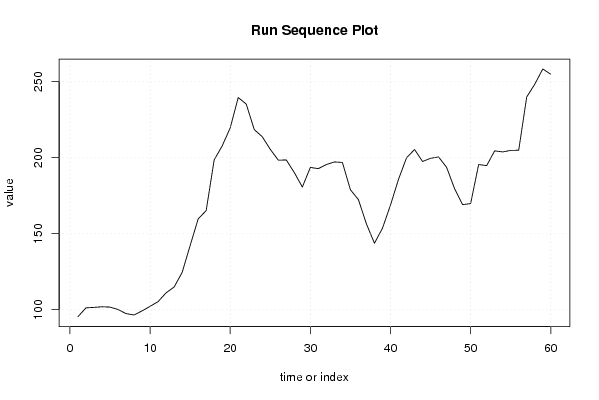
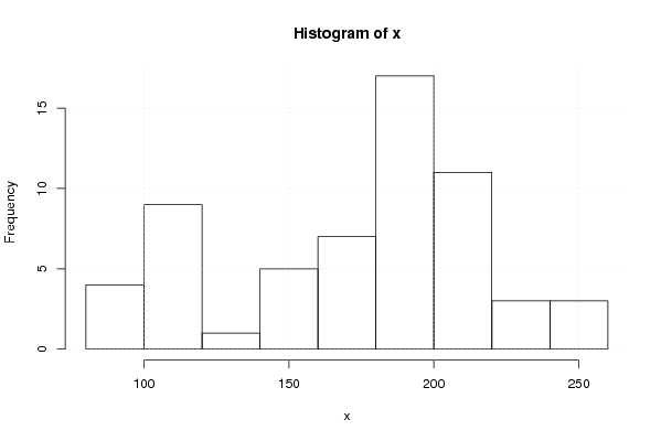
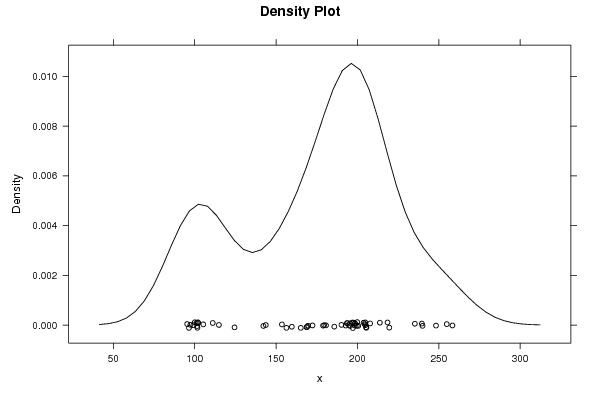
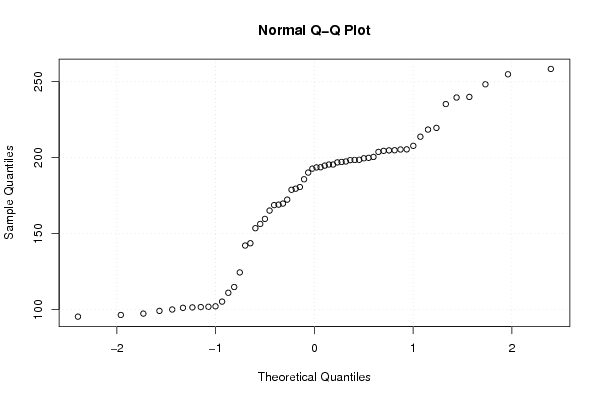
| Title produced by software | Univariate Explorative Data Analysis | ||||||||||||||||||||||||||||||||||||||||||||||||||||
| Date of computation | Mon, 27 Oct 2008 12:31:50 -0600 | ||||||||||||||||||||||||||||||||||||||||||||||||||||
| Cite this page as follows | Statistical Computations at FreeStatistics.org, Office for Research Development and Education, URL https://freestatistics.org/blog/index.php?v=date/2008/Oct/27/t1225132689y4oqpvaqwdvmns3.htm/, Retrieved Sun, 19 May 2024 15:55:49 +0000 | ||||||||||||||||||||||||||||||||||||||||||||||||||||
| Statistical Computations at FreeStatistics.org, Office for Research Development and Education, URL https://freestatistics.org/blog/index.php?pk=19388, Retrieved Sun, 19 May 2024 15:55:49 +0000 | |||||||||||||||||||||||||||||||||||||||||||||||||||||
| QR Codes: | |||||||||||||||||||||||||||||||||||||||||||||||||||||
|
| |||||||||||||||||||||||||||||||||||||||||||||||||||||
| Original text written by user: | |||||||||||||||||||||||||||||||||||||||||||||||||||||
| IsPrivate? | No (this computation is public) | ||||||||||||||||||||||||||||||||||||||||||||||||||||
| User-defined keywords | |||||||||||||||||||||||||||||||||||||||||||||||||||||
| Estimated Impact | 123 | ||||||||||||||||||||||||||||||||||||||||||||||||||||
Tree of Dependent Computations | |||||||||||||||||||||||||||||||||||||||||||||||||||||
| Family? (F = Feedback message, R = changed R code, M = changed R Module, P = changed Parameters, D = changed Data) | |||||||||||||||||||||||||||||||||||||||||||||||||||||
| F [Univariate Explorative Data Analysis] [Investigation Dis...] [2007-10-21 17:06:37] [b9964c45117f7aac638ab9056d451faa] F D [Univariate Explorative Data Analysis] [Q2 inv distr] [2008-10-24 16:12:22] [8545382734d98368249ce527c6558129] F D [Univariate Explorative Data Analysis] [steenkool] [2008-10-27 18:31:50] [1b288879226ab9a3cab0c803857233cc] [Current] - D [Univariate Explorative Data Analysis] [steenkool sept 20...] [2008-10-27 18:46:16] [8545382734d98368249ce527c6558129] | |||||||||||||||||||||||||||||||||||||||||||||||||||||
| Feedback Forum | |||||||||||||||||||||||||||||||||||||||||||||||||||||
Post a new message | |||||||||||||||||||||||||||||||||||||||||||||||||||||
Dataset | |||||||||||||||||||||||||||||||||||||||||||||||||||||
| Dataseries X: | |||||||||||||||||||||||||||||||||||||||||||||||||||||
95,4 101,2 101,5 101,9 101,7 100,1 97,4 96,5 99,2 102,2 105,3 111,1 114,9 124,5 142,2 159,7 165,2 198,6 207,8 219,6 239,6 235,3 218,5 213,8 205,5 198,4 198,5 190,2 180,7 193,6 192,8 195,5 197,2 196,9 178,9 172,4 156,4 143,7 153,6 168,8 185,8 199,9 205,4 197,5 199,6 200,5 193,7 179,6 169,1 169,8 195,5 194,8 204,5 203,8 204,8 204,9 240,0 248,3 258,4 254,9 | |||||||||||||||||||||||||||||||||||||||||||||||||||||
Tables (Output of Computation) | |||||||||||||||||||||||||||||||||||||||||||||||||||||
| |||||||||||||||||||||||||||||||||||||||||||||||||||||
Figures (Output of Computation) | |||||||||||||||||||||||||||||||||||||||||||||||||||||
Input Parameters & R Code | |||||||||||||||||||||||||||||||||||||||||||||||||||||
| Parameters (Session): | |||||||||||||||||||||||||||||||||||||||||||||||||||||
| par1 = 0 ; par2 = 0 ; | |||||||||||||||||||||||||||||||||||||||||||||||||||||
| Parameters (R input): | |||||||||||||||||||||||||||||||||||||||||||||||||||||
| par1 = 0 ; par2 = 0 ; | |||||||||||||||||||||||||||||||||||||||||||||||||||||
| R code (references can be found in the software module): | |||||||||||||||||||||||||||||||||||||||||||||||||||||
par1 <- as.numeric(par1) | |||||||||||||||||||||||||||||||||||||||||||||||||||||