Free Statistics
of Irreproducible Research!
Description of Statistical Computation | |||||||||||||||||||||||||||||||||||||
|---|---|---|---|---|---|---|---|---|---|---|---|---|---|---|---|---|---|---|---|---|---|---|---|---|---|---|---|---|---|---|---|---|---|---|---|---|---|
| Author's title | |||||||||||||||||||||||||||||||||||||
| Author | *The author of this computation has been verified* | ||||||||||||||||||||||||||||||||||||
| R Software Module | rwasp_boxcoxnorm.wasp | ||||||||||||||||||||||||||||||||||||
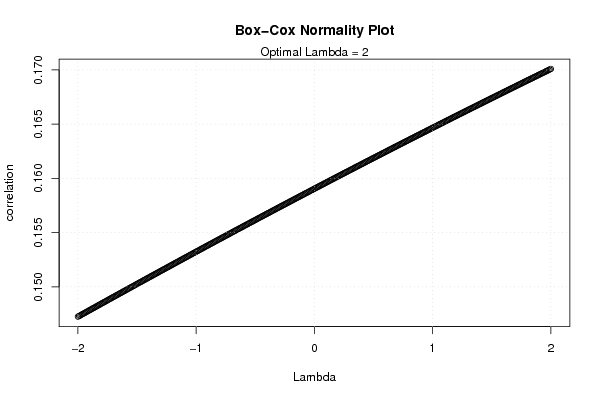
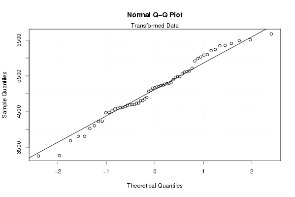
| Title produced by software | Box-Cox Normality Plot | ||||||||||||||||||||||||||||||||||||
| Date of computation | Mon, 27 Oct 2008 11:40:42 -0600 | ||||||||||||||||||||||||||||||||||||
| Cite this page as follows | Statistical Computations at FreeStatistics.org, Office for Research Development and Education, URL https://freestatistics.org/blog/index.php?v=date/2008/Oct/27/t1225129534n9brcj2b0jsr4yl.htm/, Retrieved Sun, 19 May 2024 14:57:58 +0000 | ||||||||||||||||||||||||||||||||||||
| Statistical Computations at FreeStatistics.org, Office for Research Development and Education, URL https://freestatistics.org/blog/index.php?pk=19327, Retrieved Sun, 19 May 2024 14:57:58 +0000 | |||||||||||||||||||||||||||||||||||||
| QR Codes: | |||||||||||||||||||||||||||||||||||||
|
| |||||||||||||||||||||||||||||||||||||
| Original text written by user: | |||||||||||||||||||||||||||||||||||||
| IsPrivate? | No (this computation is public) | ||||||||||||||||||||||||||||||||||||
| User-defined keywords | |||||||||||||||||||||||||||||||||||||
| Estimated Impact | 171 | ||||||||||||||||||||||||||||||||||||
Tree of Dependent Computations | |||||||||||||||||||||||||||||||||||||
| Family? (F = Feedback message, R = changed R code, M = changed R Module, P = changed Parameters, D = changed Data) | |||||||||||||||||||||||||||||||||||||
| F [Central Tendency] [Q6 Distributions] [2007-10-22 19:20:42] [b731da8b544846036771bbf9bf2f34ce] - D [Central Tendency] [Q6:Mean] [2008-10-23 11:37:05] [1ce0d16c8f4225c977b42c8fa93bc163] - RM D [Box-Cox Normality Plot] [Task 2] [2008-10-27 17:40:42] [8758b22b4a10c08c31202f233362e983] [Current] | |||||||||||||||||||||||||||||||||||||
| Feedback Forum | |||||||||||||||||||||||||||||||||||||
Post a new message | |||||||||||||||||||||||||||||||||||||
Dataset | |||||||||||||||||||||||||||||||||||||
| Dataseries X: | |||||||||||||||||||||||||||||||||||||
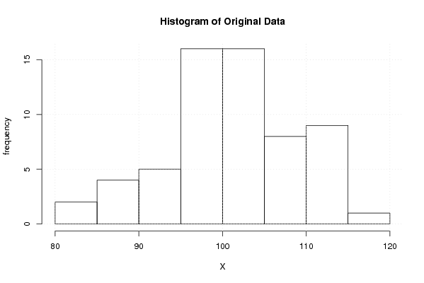
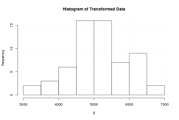
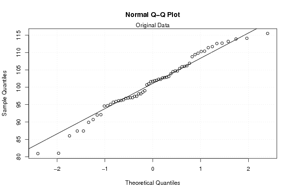
110,40 96,40 101,90 106,20 81,00 94,70 101,00 109,40 102,30 90,70 96,20 96,10 106,00 103,10 102,00 104,70 86,00 92,10 106,90 112,60 101,70 92,00 97,40 97,00 105,40 102,70 98,10 104,50 87,40 89,90 109,80 111,70 98,60 96,90 95,10 97,00 112,70 102,90 97,40 111,40 87,40 96,80 114,10 110,30 103,90 101,60 94,60 95,90 104,70 102,80 98,10 113,90 80,90 95,70 113,20 105,90 108,80 102,30 99,00 100,70 115,50 | |||||||||||||||||||||||||||||||||||||
Tables (Output of Computation) | |||||||||||||||||||||||||||||||||||||
| |||||||||||||||||||||||||||||||||||||
Figures (Output of Computation) | |||||||||||||||||||||||||||||||||||||
Input Parameters & R Code | |||||||||||||||||||||||||||||||||||||
| Parameters (Session): | |||||||||||||||||||||||||||||||||||||
| Parameters (R input): | |||||||||||||||||||||||||||||||||||||
| R code (references can be found in the software module): | |||||||||||||||||||||||||||||||||||||
n <- length(x) | |||||||||||||||||||||||||||||||||||||