Free Statistics

of Irreproducible Research!

Author's title

Author*The author of this computation has been verified*
R Software Modulerwasp_fitdistrweibull.wasp
Title produced by softwareMaximum-likelihood Fitting - Weibull Distribution
Date of computationMon, 27 Oct 2008 11:08:25 -0600
Cite this page as followsStatistical Computations at FreeStatistics.org, Office for Research Development and Education, URL https://freestatistics.org/blog/index.php?v=date/2008/Oct/27/t1225127346m474qagw454h5d6.htm/, Retrieved Sun, 19 May 2024 13:21:19 +0000
Statistical Computations at FreeStatistics.org, Office for Research Development and Education, URL https://freestatistics.org/blog/index.php?pk=19275, Retrieved Sun, 19 May 2024 13:21:19 +0000
QR Codes:

Original text written by user:
IsPrivate?No (this computation is public)
User-defined keywordstask 2 weibul
Estimated Impact164
Family? (F = Feedback message, R = changed R code, M = changed R Module, P = changed Parameters, D = changed Data)
F     [Tukey lambda PPCC Plot] [Investigating Dis...] [2007-10-21 16:01:20] [b9964c45117f7aac638ab9056d451faa]
F    D  [Tukey lambda PPCC Plot] [Q1: Tukey lambda ...] [2008-10-26 12:32:26] [fe7291e888d31b8c4db0b24d6c0f75c6]
- RMP       [Maximum-likelihood Fitting - Weibull Distribution] [task 2 weibul] [2008-10-27 17:08:25] [783db4b4a0f63b73ca8b14666b7f4329] [Current]
Feedback Forum

Post a new message
Dataseries X:
110.40
96.40
101.90
106.20
81.00
94.70
101.00
109.40
102.30
90.70
96.20
96.10
106.00
103.10
102.00
104.70
86.00
92.10
106.90
112.60
101.70
92.00
97.40
97.00
105.40
102.70
98.10
104.50
87.40
89.90
109.80
111.70
98.60
96.90
95.10
97.00
112.70
102.90
97.40
111.40
87.40
96.80
114.10
110.30
103.90
101.60
94.60
95.90
104.70
102.80
98.10
113.90
80.90
95.70
113.20
105.90
108.80
102.30
99.00
100.70
115.50


Summary of computational transaction
Raw Inputview raw input (R code)
Raw Outputview raw output of R engine
Computing time1 seconds
R Server'Gwilym Jenkins' @ 72.249.127.135

\begin{tabular}{lllllllll}
\hline
Summary of computational transaction \tabularnewline
Raw Input & view raw input (R code)  \tabularnewline
Raw Output & view raw output of R engine  \tabularnewline
Computing time & 1 seconds \tabularnewline
R Server & 'Gwilym Jenkins' @ 72.249.127.135 \tabularnewline
\hline
\end{tabular}
%Source: https://freestatistics.org/blog/index.php?pk=19275&T=0

[TABLE]
[ROW][C]Summary of computational transaction[/C][/ROW]
[ROW][C]Raw Input[/C][C]view raw input (R code) [/C][/ROW]
[ROW][C]Raw Output[/C][C]view raw output of R engine [/C][/ROW]
[ROW][C]Computing time[/C][C]1 seconds[/C][/ROW]
[ROW][C]R Server[/C][C]'Gwilym Jenkins' @ 72.249.127.135[/C][/ROW]
[/TABLE]
Source: https://freestatistics.org/blog/index.php?pk=19275&T=0

Globally Unique Identifier (entire table): ba.freestatistics.org/blog/index.php?pk=19275&T=0

As an alternative you can also use a QR Code:  

The GUIDs for individual cells are displayed in the table below:

Summary of computational transaction
Raw Inputview raw input (R code)
Raw Outputview raw output of R engine
Computing time1 seconds
R Server'Gwilym Jenkins' @ 72.249.127.135


ParameterEstimated ValueStandard Deviation
shape14.45904602587431.42791167778649
scale104.5355467241570.978118926258692

\begin{tabular}{lllllllll}
\hline
Parameter & Estimated Value & Standard Deviation \tabularnewline
shape & 14.4590460258743 & 1.42791167778649 \tabularnewline
scale & 104.535546724157 & 0.978118926258692 \tabularnewline
\hline
\end{tabular}
%Source: https://freestatistics.org/blog/index.php?pk=19275&T=1

[TABLE]
[ROW][C]Parameter[/C][C]Estimated Value[/C][C]Standard Deviation[/C][/ROW]
[ROW][C]shape[/C][C]14.4590460258743[/C][C]1.42791167778649[/C][/ROW]
[ROW][C]scale[/C][C]104.535546724157[/C][C]0.978118926258692[/C][/ROW]
[/TABLE]
Source: https://freestatistics.org/blog/index.php?pk=19275&T=1

Globally Unique Identifier (entire table): ba.freestatistics.org/blog/index.php?pk=19275&T=1

As an alternative you can also use a QR Code:  

The GUIDs for individual cells are displayed in the table below:

ParameterEstimated ValueStandard Deviation
shape14.45904602587431.42791167778649
scale104.5355467241570.978118926258692


Parameters (Session):
par1 = 1 ; par2 = 8 ;
Parameters (R input):
par1 = 1 ; par2 = 8 ;
R code (references can be found in the software module):
library(MASS)
PPCCWeibull <- function(shape, scale, x)
{
x <- sort(x)
pp <- ppoints(x)
cor(qweibull(pp, shape=shape, scale=scale), x)
}
par1 <- as.numeric(par1)
par2 <- as.numeric(par2)
if (par1 < 0.1) par1 <- 0.1
if (par1 > 50) par1 <- 50
if (par2 < 0.1) par2 <- 0.1
if (par2 > 50) par2 <- 50
par1h <- par1*10
par2h <- par2*10
sortx <- sort(x)
c <- array(NA,dim=c(par2h))
for (i in par1h:par2h)
{
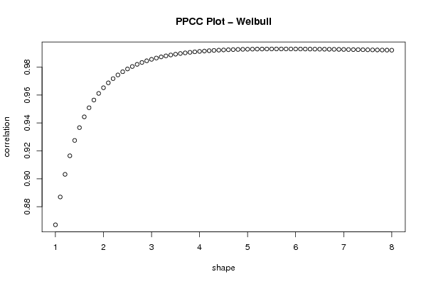
c[i] <- cor(qweibull(ppoints(x), shape=i/10,scale=2),sortx)
}
bitmap(file='test1.png')
plot((par1h:par2h)/10,c[par1h:par2h],xlab='shape',ylab='correlation',main='PPCC Plot - Weibull')
dev.off()
f<-fitdistr(x, 'weibull')
f$estimate
f$sd
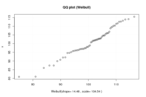
xlab <- paste('Weibull(shape=',round(f$estimate[[1]],2))
xlab <- paste(xlab,', scale=')
xlab <- paste(xlab,round(f$estimate[[2]],2))
xlab <- paste(xlab,')')
bitmap(file='test2.png')
qqplot(qweibull(ppoints(x), shape=f$estimate[[1]], scale=f$estimate[[2]]), x, main='QQ plot (Weibull)', xlab=xlab )
grid()
dev.off()
load(file='createtable')
a<-table.start()
a<-table.row.start(a)
a<-table.element(a,'Parameter',1,TRUE)
a<-table.element(a,'Estimated Value',1,TRUE)
a<-table.element(a,'Standard Deviation',1,TRUE)
a<-table.row.end(a)
a<-table.row.start(a)
a<-table.element(a,'shape',header=TRUE)
a<-table.element(a,f$estimate[1])
a<-table.element(a,f$sd[1])
a<-table.row.end(a)
a<-table.row.start(a)
a<-table.element(a,'scale',header=TRUE)
a<-table.element(a,f$estimate[2])
a<-table.element(a,f$sd[2])
a<-table.row.end(a)
a<-table.end(a)
table.save(a,file='mytable.tab')