Free Statistics
of Irreproducible Research!
Description of Statistical Computation | |||||||||||||||||||||||||||||||||||||||||||||||||||||
|---|---|---|---|---|---|---|---|---|---|---|---|---|---|---|---|---|---|---|---|---|---|---|---|---|---|---|---|---|---|---|---|---|---|---|---|---|---|---|---|---|---|---|---|---|---|---|---|---|---|---|---|---|---|
| Author's title | |||||||||||||||||||||||||||||||||||||||||||||||||||||
| Author | *The author of this computation has been verified* | ||||||||||||||||||||||||||||||||||||||||||||||||||||
| R Software Module | rwasp_edauni.wasp | ||||||||||||||||||||||||||||||||||||||||||||||||||||
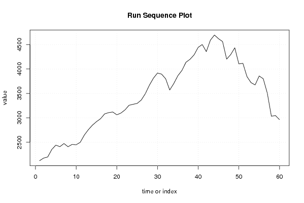
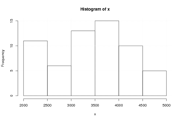
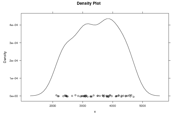
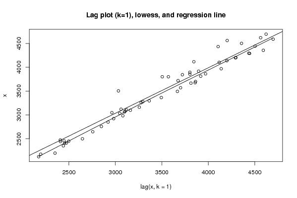
| Title produced by software | Univariate Explorative Data Analysis | ||||||||||||||||||||||||||||||||||||||||||||||||||||
| Date of computation | Mon, 27 Oct 2008 03:27:49 -0600 | ||||||||||||||||||||||||||||||||||||||||||||||||||||
| Cite this page as follows | Statistical Computations at FreeStatistics.org, Office for Research Development and Education, URL https://freestatistics.org/blog/index.php?v=date/2008/Oct/27/t1225099765xh8vbokpudb1ftu.htm/, Retrieved Sun, 19 May 2024 12:58:03 +0000 | ||||||||||||||||||||||||||||||||||||||||||||||||||||
| Statistical Computations at FreeStatistics.org, Office for Research Development and Education, URL https://freestatistics.org/blog/index.php?pk=19136, Retrieved Sun, 19 May 2024 12:58:03 +0000 | |||||||||||||||||||||||||||||||||||||||||||||||||||||
| QR Codes: | |||||||||||||||||||||||||||||||||||||||||||||||||||||
|
| |||||||||||||||||||||||||||||||||||||||||||||||||||||
| Original text written by user: | |||||||||||||||||||||||||||||||||||||||||||||||||||||
| IsPrivate? | No (this computation is public) | ||||||||||||||||||||||||||||||||||||||||||||||||||||
| User-defined keywords | |||||||||||||||||||||||||||||||||||||||||||||||||||||
| Estimated Impact | 190 | ||||||||||||||||||||||||||||||||||||||||||||||||||||
Tree of Dependent Computations | |||||||||||||||||||||||||||||||||||||||||||||||||||||
| Family? (F = Feedback message, R = changed R code, M = changed R Module, P = changed Parameters, D = changed Data) | |||||||||||||||||||||||||||||||||||||||||||||||||||||
| F [Univariate Data Series] [Beurskoers Eurone...] [2008-10-13 22:20:32] [82970caad4b026be9dd352fdec547fe4] - PD [Univariate Data Series] [Beurskoers Eurone...] [2008-10-20 20:09:06] [82970caad4b026be9dd352fdec547fe4] F RMP [Univariate Explorative Data Analysis] [Investigating Dis...] [2008-10-27 09:27:49] [c33ddd06d9ea3933c8ac89c0e74c9b3a] [Current] F RMP [Tukey lambda PPCC Plot] [Investigating Dis...] [2008-10-27 10:05:32] [82970caad4b026be9dd352fdec547fe4] - [Tukey lambda PPCC Plot] [Investigating Dis...] [2008-11-03 08:50:35] [38f43994ada0e6172896e12525dcc585] F RMP [Harrell-Davis Quantiles] [Investigating Dis...] [2008-10-27 10:20:53] [82970caad4b026be9dd352fdec547fe4] - P [Univariate Explorative Data Analysis] [Verbetering Q7 va...] [2008-10-30 14:13:28] [73d6180dc45497329efd1b6934a84aba] - PD [Univariate Explorative Data Analysis] [Investigating Dis...] [2008-11-03 08:22:22] [38f43994ada0e6172896e12525dcc585] | |||||||||||||||||||||||||||||||||||||||||||||||||||||
| Feedback Forum | |||||||||||||||||||||||||||||||||||||||||||||||||||||
Post a new message | |||||||||||||||||||||||||||||||||||||||||||||||||||||
Dataset | |||||||||||||||||||||||||||||||||||||||||||||||||||||
| Dataseries X: | |||||||||||||||||||||||||||||||||||||||||||||||||||||
2120.88 2174.56 2196.72 2350.44 2440.25 2408.64 2472.81 2407.6 2454.62 2448.05 2497.84 2645.64 2756.76 2849.27 2921.44 2981.85 3080.58 3106.22 3119.31 3061.26 3097.31 3161.69 3257.16 3277.01 3295.32 3363.99 3494.17 3667.03 3813.06 3917.96 3895.51 3801.06 3570.12 3701.61 3862.27 3970.1 4138.52 4199.75 4290.89 4443.91 4502.64 4356.98 4591.27 4696.96 4621.4 4562.84 4202.52 4296.49 4435.23 4105.18 4116.68 3844.49 3720.98 3674.4 3857.62 3801.06 3504.37 3032.6 3047.03 2962.34 | |||||||||||||||||||||||||||||||||||||||||||||||||||||
Tables (Output of Computation) | |||||||||||||||||||||||||||||||||||||||||||||||||||||
| |||||||||||||||||||||||||||||||||||||||||||||||||||||
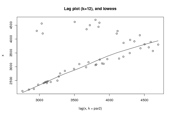
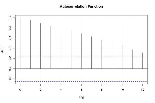
Figures (Output of Computation) | |||||||||||||||||||||||||||||||||||||||||||||||||||||
Input Parameters & R Code | |||||||||||||||||||||||||||||||||||||||||||||||||||||
| Parameters (Session): | |||||||||||||||||||||||||||||||||||||||||||||||||||||
| par1 = 0 ; par2 = 12 ; | |||||||||||||||||||||||||||||||||||||||||||||||||||||
| Parameters (R input): | |||||||||||||||||||||||||||||||||||||||||||||||||||||
| par1 = 0 ; par2 = 12 ; | |||||||||||||||||||||||||||||||||||||||||||||||||||||
| R code (references can be found in the software module): | |||||||||||||||||||||||||||||||||||||||||||||||||||||
par1 <- as.numeric(par1) | |||||||||||||||||||||||||||||||||||||||||||||||||||||