Repository of Reproducible Computations

Free Statistics

of Irreproducible Research!

Author's title

Author

*The author of this computation has been verified*

R Software Module

rwasp_edauni.wasp

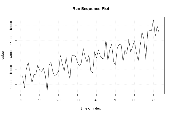
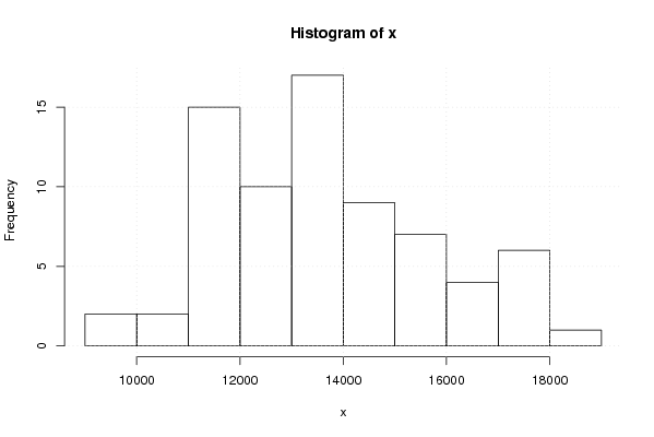
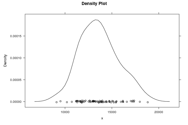
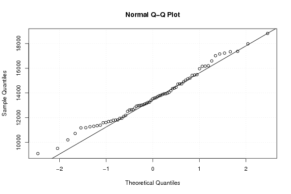
Title produced by software

Univariate Explorative Data Analysis

Date of computation

Sat, 25 Oct 2008 08:50:53 -0600

Cite this page as follows

Statistical Computations at FreeStatistics.org, Office for Research Development and Education, URL https://freestatistics.org/blog/index.php?v=date/2008/Oct/25/t1224946335ropp14zg4qco1o0.htm/, Retrieved Sun, 19 May 2024 15:54:53 +0000

Statistical Computations at FreeStatistics.org, Office for Research Development and Education, URL https://freestatistics.org/blog/index.php?pk=18761, Retrieved Sun, 19 May 2024 15:54:53 +0000

QR Codes:

Paste this QR Code to cite your computation.

Original text written by user:

IsPrivate?

No (this computation is public)

User-defined keywords

seasonality uitvoer europa

Estimated Impact

139

Family? (F = Feedback message, R = changed R code, M = changed R Module, P = changed Parameters, D = changed Data)

F       [Univariate Explorative Data Analysis] [Seasonality Uitvo...] [2008-10-25 14:50:53] [8da7502cfecb272886bc60b3f290b8b8] [Current]
- RMPD    [Mean Plot] [Mean plot] [2008-11-03 18:29:33] [e7f730ba3fad917ffc21bb9e72c10880] 

Feedback Forum

2008-11-04 07:39:09 [Koen De Winter] [reply] 
Ik heb een nieuwe berekening gemaakt met de mean plot, omdat je hierop beter seizoensgebondenheid kan terugvinden.  
 
http://www.freestatistics.org/blog/date/2008/Nov/03/t12257370340nj93zwxbt5kmzu.htm 
 
Ik stel met die techniek vast dat er wel sprake is van een terugkerend patroon. De seizoensgebondenheid is er niet uitdrukkelijk en door de stijgende trend moeilijker te herkennen, toch vind ik ze voor discussie waard. Kijk maar naar de dieptepunten bij 12, 24, 36, 48, 60 en 72.

Post a new message

Dataseries X:

Download CSV

Histogram

Boxplots

Summary of computational transaction
Raw Input	view raw input (R code)
Raw Output	view raw output of R engine
Computing time	4 seconds
R Server	'Sir Ronald Aylmer Fisher' @ 193.190.124.24

\begin{tabular}{lllllllll}
\hline
Summary of computational transaction \tabularnewline
Raw Input & view raw input (R code)  \tabularnewline
Raw Output & view raw output of R engine  \tabularnewline
Computing time & 4 seconds \tabularnewline
R Server & 'Sir Ronald Aylmer Fisher' @ 193.190.124.24 \tabularnewline
\hline
\end{tabular}
%Source: https://freestatistics.org/blog/index.php?pk=18761&T=0

[TABLE]
[ROW][C]Summary of computational transaction[/C][/ROW]
[ROW][C]Raw Input[/C][C]view raw input (R code) [/C][/ROW]
[ROW][C]Raw Output[/C][C]view raw output of R engine [/C][/ROW]
[ROW][C]Computing time[/C][C]4 seconds[/C][/ROW]
[ROW][C]R Server[/C][C]'Sir Ronald Aylmer Fisher' @ 193.190.124.24[/C][/ROW]
[/TABLE]
Source: https://freestatistics.org/blog/index.php?pk=18761&T=0

Globally Unique Identifier (entire table): ba.freestatistics.org/blog/index.php?pk=18761&T=0

As an alternative you can also use a QR Code:

The GUIDs for individual cells are displayed in the table below:

Summary of computational transaction
Raw Input	view raw input (R code)
Raw Output	view raw output of R engine
Computing time	4 seconds
R Server	'Sir Ronald Aylmer Fisher' @ 193.190.124.24

Descriptive Statistics
# observations	73
minimum	9097.4
Q1	11956.6
median	13527.5
mean	13640.7287671233
Q3	14908.3
maximum	18817.8

\begin{tabular}{lllllllll}
\hline
Descriptive Statistics \tabularnewline
# observations & 73 \tabularnewline
minimum & 9097.4 \tabularnewline
Q1 & 11956.6 \tabularnewline
median & 13527.5 \tabularnewline
mean & 13640.7287671233 \tabularnewline
Q3 & 14908.3 \tabularnewline
maximum & 18817.8 \tabularnewline
\hline
\end{tabular}
%Source: https://freestatistics.org/blog/index.php?pk=18761&T=1

[TABLE]
[ROW][C]Descriptive Statistics[/C][/ROW]
[ROW][C]# observations[/C][C]73[/C][/ROW]
[ROW][C]minimum[/C][C]9097.4[/C][/ROW]
[ROW][C]Q1[/C][C]11956.6[/C][/ROW]
[ROW][C]median[/C][C]13527.5[/C][/ROW]
[ROW][C]mean[/C][C]13640.7287671233[/C][/ROW]
[ROW][C]Q3[/C][C]14908.3[/C][/ROW]
[ROW][C]maximum[/C][C]18817.8[/C][/ROW]
[/TABLE]
Source: https://freestatistics.org/blog/index.php?pk=18761&T=1

Globally Unique Identifier (entire table): ba.freestatistics.org/blog/index.php?pk=18761&T=1

As an alternative you can also use a QR Code:

The GUIDs for individual cells are displayed in the table below:

Descriptive Statistics
# observations	73
minimum	9097.4
Q1	11956.6
median	13527.5
mean	13640.7287671233
Q3	14908.3
maximum	18817.8

Figure 1

PNG link

Postscript link

PDF link

Figure 2

PNG link

Postscript link

PDF link

Figure 3

PNG link

Postscript link

PDF link

Figure 4

PNG link

Postscript link

PDF link

Figure 5

PNG link

Postscript link

PDF link

Figure 6

PNG link

Postscript link

PDF link

Figure 7

PNG link

Postscript link

PDF link

Parameters (Session):

par1 = 0 ; par2 = 0 ;

Parameters (R input):

par1 = 0 ; par2 = 0 ;

R code (references can be found in the software module):

par1 <- as.numeric(par1)
par2 <- as.numeric(par2)
x <- as.ts(x)
library(lattice)
bitmap(file='pic1.png')
plot(x,type='l',main='Run Sequence Plot',xlab='time or index',ylab='value')
grid()
dev.off()
bitmap(file='pic2.png')
hist(x)
grid()
dev.off()
bitmap(file='pic3.png')
if (par1 > 0)
{
densityplot(~x,col='black',main=paste('Density Plot   bw = ',par1),bw=par1)
} else {
densityplot(~x,col='black',main='Density Plot')
}
dev.off()
bitmap(file='pic4.png')
qqnorm(x)
qqline(x)
grid()
dev.off()
if (par2 > 0)
{
bitmap(file='lagplot1.png')
dum <- cbind(lag(x,k=1),x)
dum
dum1 <- dum[2:length(x),]
dum1
z <- as.data.frame(dum1)
z
plot(z,main='Lag plot (k=1), lowess, and regression line')
lines(lowess(z))
abline(lm(z))
dev.off()
if (par2 > 1) {
bitmap(file='lagplotpar2.png')
dum <- cbind(lag(x,k=par2),x)
dum
dum1 <- dum[(par2+1):length(x),]
dum1
z <- as.data.frame(dum1)
z
mylagtitle <- 'Lag plot (k='
mylagtitle <- paste(mylagtitle,par2,sep='')
mylagtitle <- paste(mylagtitle,'), and lowess',sep='')
plot(z,main=mylagtitle)
lines(lowess(z))
dev.off()
}
bitmap(file='pic5.png')
acf(x,lag.max=par2,main='Autocorrelation Function')
grid()
dev.off()
}
summary(x)
load(file='createtable')
a<-table.start()
a<-table.row.start(a)
a<-table.element(a,'Descriptive Statistics',2,TRUE)
a<-table.row.end(a)
a<-table.row.start(a)
a<-table.element(a,'# observations',header=TRUE)
a<-table.element(a,length(x))
a<-table.row.end(a)
a<-table.row.start(a)
a<-table.element(a,'minimum',header=TRUE)
a<-table.element(a,min(x))
a<-table.row.end(a)
a<-table.row.start(a)
a<-table.element(a,'Q1',header=TRUE)
a<-table.element(a,quantile(x,0.25))
a<-table.row.end(a)
a<-table.row.start(a)
a<-table.element(a,'median',header=TRUE)
a<-table.element(a,median(x))
a<-table.row.end(a)
a<-table.row.start(a)
a<-table.element(a,'mean',header=TRUE)
a<-table.element(a,mean(x))
a<-table.row.end(a)
a<-table.row.start(a)
a<-table.element(a,'Q3',header=TRUE)
a<-table.element(a,quantile(x,0.75))
a<-table.row.end(a)
a<-table.row.start(a)
a<-table.element(a,'maximum',header=TRUE)
a<-table.element(a,max(x))
a<-table.row.end(a)
a<-table.end(a)
table.save(a,file='mytable.tab')

Free Statistics

Description of Statistical Computation

Tree of Dependent Computations

Dataset

Tables (Output of Computation)

Figures (Output of Computation)

Input Parameters & R Code