Free Statistics
of Irreproducible Research!
Description of Statistical Computation | |||||||||||||||||||||||||||||||||||||||||||||||||||||
|---|---|---|---|---|---|---|---|---|---|---|---|---|---|---|---|---|---|---|---|---|---|---|---|---|---|---|---|---|---|---|---|---|---|---|---|---|---|---|---|---|---|---|---|---|---|---|---|---|---|---|---|---|---|
| Author's title | |||||||||||||||||||||||||||||||||||||||||||||||||||||
| Author | *The author of this computation has been verified* | ||||||||||||||||||||||||||||||||||||||||||||||||||||
| R Software Module | rwasp_edauni.wasp | ||||||||||||||||||||||||||||||||||||||||||||||||||||
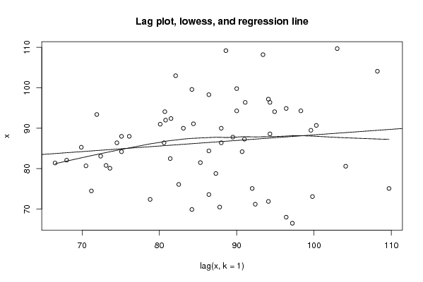
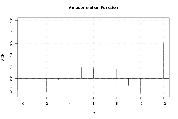
| Title produced by software | Univariate Explorative Data Analysis | ||||||||||||||||||||||||||||||||||||||||||||||||||||
| Date of computation | Fri, 24 Oct 2008 07:12:07 -0600 | ||||||||||||||||||||||||||||||||||||||||||||||||||||
| Cite this page as follows | Statistical Computations at FreeStatistics.org, Office for Research Development and Education, URL https://freestatistics.org/blog/index.php?v=date/2008/Oct/24/t1224861234k2oolop40y48cx4.htm/, Retrieved Tue, 28 May 2024 17:34:19 +0000 | ||||||||||||||||||||||||||||||||||||||||||||||||||||
| Statistical Computations at FreeStatistics.org, Office for Research Development and Education, URL https://freestatistics.org/blog/index.php?pk=18636, Retrieved Tue, 28 May 2024 17:34:19 +0000 | |||||||||||||||||||||||||||||||||||||||||||||||||||||
| QR Codes: | |||||||||||||||||||||||||||||||||||||||||||||||||||||
|
| |||||||||||||||||||||||||||||||||||||||||||||||||||||
| Original text written by user: | |||||||||||||||||||||||||||||||||||||||||||||||||||||
| IsPrivate? | No (this computation is public) | ||||||||||||||||||||||||||||||||||||||||||||||||||||
| User-defined keywords | |||||||||||||||||||||||||||||||||||||||||||||||||||||
| Estimated Impact | 186 | ||||||||||||||||||||||||||||||||||||||||||||||||||||
Tree of Dependent Computations | |||||||||||||||||||||||||||||||||||||||||||||||||||||
| Family? (F = Feedback message, R = changed R code, M = changed R Module, P = changed Parameters, D = changed Data) | |||||||||||||||||||||||||||||||||||||||||||||||||||||
| F [Univariate Explorative Data Analysis] [Investigation Dis...] [2007-10-21 17:06:37] [b9964c45117f7aac638ab9056d451faa] F PD [Univariate Explorative Data Analysis] [herberekening vra...] [2008-10-24 13:12:07] [3dc594a6c62226e1e98766c4d385bfaa] [Current] F D [Univariate Explorative Data Analysis] [vraag 7] [2008-10-26 11:17:02] [c45c87b96bbf32ffc2144fc37d767b2e] - P [Univariate Explorative Data Analysis] [verbetering taak 3] [2008-11-02 12:24:26] [c45c87b96bbf32ffc2144fc37d767b2e] - RMPD [Pearson Correlation] [correlatie rnvm -...] [2008-10-30 11:34:51] [28075c6928548bea087cb2be962cfe7e] F RM D [Kendall tau Correlation Matrix] [Q1] [2008-10-30 12:28:36] [28075c6928548bea087cb2be962cfe7e] - RMPD [Pearson Correlation] [correlatie rcf - rnr] [2008-10-30 11:37:41] [28075c6928548bea087cb2be962cfe7e] - RMPD [Pearson Correlation] [correlatie tussen...] [2008-10-30 11:41:51] [28075c6928548bea087cb2be962cfe7e] - RMPD [Pearson Correlation] [correlatie ren en...] [2008-10-30 11:44:13] [28075c6928548bea087cb2be962cfe7e] F RMPD [Star Plot] [q2] [2008-10-30 11:52:06] [28075c6928548bea087cb2be962cfe7e] F RMPD [Notched Boxplots] [notch boxplot Q3] [2008-10-30 12:09:20] [28075c6928548bea087cb2be962cfe7e] F P [Univariate Explorative Data Analysis] [vraag 5] [2008-11-11 15:06:24] [c45c87b96bbf32ffc2144fc37d767b2e] | |||||||||||||||||||||||||||||||||||||||||||||||||||||
| Feedback Forum | |||||||||||||||||||||||||||||||||||||||||||||||||||||
Post a new message | |||||||||||||||||||||||||||||||||||||||||||||||||||||
Dataset | |||||||||||||||||||||||||||||||||||||||||||||||||||||
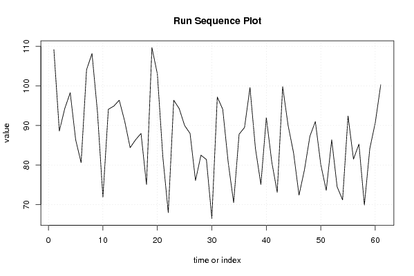
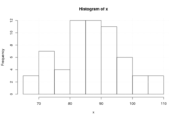
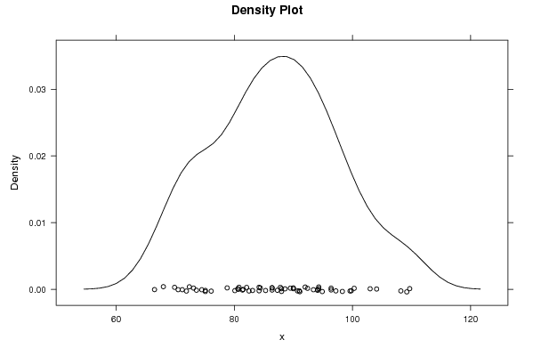
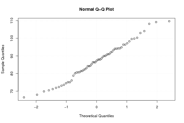
| Dataseries X: | |||||||||||||||||||||||||||||||||||||||||||||||||||||
109.20 88.60 94.30 98.30 86.40 80.60 104.10 108.20 93.40 71.90 94.10 94.90 96.40 91.10 84.40 86.40 88.00 75.10 109.70 103.00 82.10 68.00 96.40 94.30 90.00 88.00 76.10 82.50 81.40 66.50 97.20 94.10 80.70 70.50 87.80 89.50 99.60 84.20 75.10 92.00 80.80 73.10 99.80 90.00 83.10 72.40 78.80 87.30 91.00 80.10 73.60 86.40 74.50 71.20 92.40 81.50 85.30 69.90 84.20 90.70 100.30 | |||||||||||||||||||||||||||||||||||||||||||||||||||||
Tables (Output of Computation) | |||||||||||||||||||||||||||||||||||||||||||||||||||||
| |||||||||||||||||||||||||||||||||||||||||||||||||||||
Figures (Output of Computation) | |||||||||||||||||||||||||||||||||||||||||||||||||||||
Input Parameters & R Code | |||||||||||||||||||||||||||||||||||||||||||||||||||||
| Parameters (Session): | |||||||||||||||||||||||||||||||||||||||||||||||||||||
| par1 = 0 ; par2 = 12 ; | |||||||||||||||||||||||||||||||||||||||||||||||||||||
| Parameters (R input): | |||||||||||||||||||||||||||||||||||||||||||||||||||||
| par1 = 0 ; par2 = 12 ; | |||||||||||||||||||||||||||||||||||||||||||||||||||||
| R code (references can be found in the software module): | |||||||||||||||||||||||||||||||||||||||||||||||||||||
par1 <- as.numeric(par1) | |||||||||||||||||||||||||||||||||||||||||||||||||||||