Repository of Reproducible Computations

Free Statistics

of Irreproducible Research!

Author's title

Author

*The author of this computation has been verified*

R Software Module

rwasp_tukeylambda.wasp

Title produced by software

Tukey lambda PPCC Plot

Date of computation

Fri, 24 Oct 2008 07:18:16 -0600

Cite this page as follows

Statistical Computations at FreeStatistics.org, Office for Research Development and Education, URL https://freestatistics.org/blog/index.php?v=date/2008/Oct/24/t1224854369h89a9e0v4ffppqj.htm/, Retrieved Sun, 19 May 2024 15:23:19 +0000

Statistical Computations at FreeStatistics.org, Office for Research Development and Education, URL https://freestatistics.org/blog/index.php?pk=18603, Retrieved Sun, 19 May 2024 15:23:19 +0000

QR Codes:

Paste this QR Code to cite your computation.

Original text written by user:

IsPrivate?

No (this computation is public)

User-defined keywords

Estimated Impact

203

Family? (F = Feedback message, R = changed R code, M = changed R Module, P = changed Parameters, D = changed Data)

F     [Tukey lambda PPCC Plot] [Investigating Dis...] [2007-10-21 16:01:20] [b9964c45117f7aac638ab9056d451faa]
F    D    [Tukey lambda PPCC Plot] [PPCC - tukey lambda] [2008-10-24 13:18:16] [de3f0516a1536f7c4a656924d8bc8d07] [Current]

Feedback Forum

2008-10-29 15:47:47 [Nathalie Koulouris] [reply] 
De student heeft gebruik gemaakt van de juiste methode want de hoogste correlatiewaarde wordt inderdaad teruggevonden bij de normaalverdeling.
2008-11-01 13:22:58 [Kristof Augustyns] [reply] 
Er is hier inderdaad gebruik gemaakt van een juiste berekening. 
Bij een normaal verdeling (lambda 0,14) bekomt men de hoogste correlatie. 
0.989505916159088 is die correlatie en staat dus op 1/100 ste van de '1'. 
Hoe normaler, hoe hoger de correlatie. 
2008-11-01 13:47:54 [Kim Huysmans] [reply] 
Het klopt inderdaad dat we hier een normale verdeling hebben. Als we gaan kijken waarom deze normaal verdeling zo belangrijk is komen we tot een belangrijke wetmatigheid van de statistiek. We nemen elk punt in een gegeven tijdreeks als een steekproef van 1 observatie. Wanneer deze punten onafhankelijk zijn van elkaar, zijn deze opeenvolgende punten steeds normaal verdeeld zijn. De punten zijn onafhankelijk van elkaar als er geen autocorrelatie is.
2008-11-01 20:37:34 [Steffi Van Isveldt] [reply] 
De normaalverdeling is vooral belangrijk omdat we pas bij zo'n verdeling correcte uitspraken kunnen doen over onze reeksen.
2008-11-03 10:29:21 [Karen Van den Broeck] [reply] 
De student heeft dit goed opgelost. De hoogste correlatiewaarde vinden we bij Approx.Normal. Deze ligt dicht tegen 1 en dit houdt in dat de tijdreeks een normaalverdeling heeft. Waarom is deze normaalverdeling van belang? O.b.v. steekproeven iets zeggen over de totala populatie. We nemen elk punt in gegeven tijdreeks als steekproef van 1 observatie. Deze punten moeten onafhankelijk zijn van elkaar en wanneer dit het geval is, zijn de opeenvolgende punten normaal verdeeld. Onafhankelijk is hier het belangrijkst(dus geen autocorrelatie).

Post a new message

Dataseries X:

Download CSV

Histogram

Boxplots

Summary of computational transaction
Raw Input	view raw input (R code)
Raw Output	view raw output of R engine
Computing time	3 seconds
R Server	'Herman Ole Andreas Wold' @ 193.190.124.10:1001

\begin{tabular}{lllllllll}
\hline
Summary of computational transaction \tabularnewline
Raw Input & view raw input (R code)  \tabularnewline
Raw Output & view raw output of R engine  \tabularnewline
Computing time & 3 seconds \tabularnewline
R Server & 'Herman Ole Andreas Wold' @ 193.190.124.10:1001 \tabularnewline
\hline
\end{tabular}
%Source: https://freestatistics.org/blog/index.php?pk=18603&T=0

[TABLE]
[ROW][C]Summary of computational transaction[/C][/ROW]
[ROW][C]Raw Input[/C][C]view raw input (R code) [/C][/ROW]
[ROW][C]Raw Output[/C][C]view raw output of R engine [/C][/ROW]
[ROW][C]Computing time[/C][C]3 seconds[/C][/ROW]
[ROW][C]R Server[/C][C]'Herman Ole Andreas Wold' @ 193.190.124.10:1001[/C][/ROW]
[/TABLE]
Source: https://freestatistics.org/blog/index.php?pk=18603&T=0

Globally Unique Identifier (entire table): ba.freestatistics.org/blog/index.php?pk=18603&T=0

As an alternative you can also use a QR Code:

The GUIDs for individual cells are displayed in the table below:

Summary of computational transaction
Raw Input	view raw input (R code)
Raw Output	view raw output of R engine
Computing time	3 seconds
R Server	'Herman Ole Andreas Wold' @ 193.190.124.10:1001

Tukey Lambda - Key Values
Distribution (lambda)	Correlation
Approx. Cauchy (lambda=-1)	0.681034394717584
Exact Logistic (lambda=0)	0.984820721672163
Approx. Normal (lambda=0.14)	0.989505916159088
U-shaped (lambda=0.5)	0.985385537255734
Exactly Uniform (lambda=1)	0.97511352322751

\begin{tabular}{lllllllll}
\hline
Tukey Lambda - Key Values \tabularnewline
Distribution (lambda) & Correlation \tabularnewline
Approx. Cauchy (lambda=-1) & 0.681034394717584 \tabularnewline
Exact Logistic (lambda=0) & 0.984820721672163 \tabularnewline
Approx. Normal (lambda=0.14) & 0.989505916159088 \tabularnewline
U-shaped (lambda=0.5) & 0.985385537255734 \tabularnewline
Exactly Uniform (lambda=1) & 0.97511352322751 \tabularnewline
\hline
\end{tabular}
%Source: https://freestatistics.org/blog/index.php?pk=18603&T=1

[TABLE]
[ROW][C]Tukey Lambda - Key Values[/C][/ROW]
[ROW][C]Distribution (lambda)[/C][C]Correlation[/C][/ROW]
[ROW][C]Approx. Cauchy (lambda=-1)[/C][C]0.681034394717584[/C][/ROW]
[ROW][C]Exact Logistic (lambda=0)[/C][C]0.984820721672163[/C][/ROW]
[ROW][C]Approx. Normal (lambda=0.14)[/C][C]0.989505916159088[/C][/ROW]
[ROW][C]U-shaped (lambda=0.5)[/C][C]0.985385537255734[/C][/ROW]
[ROW][C]Exactly Uniform (lambda=1)[/C][C]0.97511352322751[/C][/ROW]
[/TABLE]
Source: https://freestatistics.org/blog/index.php?pk=18603&T=1

Globally Unique Identifier (entire table): ba.freestatistics.org/blog/index.php?pk=18603&T=1

As an alternative you can also use a QR Code:

The GUIDs for individual cells are displayed in the table below:

Tukey Lambda - Key Values
Distribution (lambda)	Correlation
Approx. Cauchy (lambda=-1)	0.681034394717584
Exact Logistic (lambda=0)	0.984820721672163
Approx. Normal (lambda=0.14)	0.989505916159088
U-shaped (lambda=0.5)	0.985385537255734
Exactly Uniform (lambda=1)	0.97511352322751

Figure 1

PNG link

Postscript link

PDF link

Parameters (Session):

Parameters (R input):

R code (references can be found in the software module):

gp <- function(lambda, p)
{
(p^lambda-(1-p)^lambda)/lambda
}
sortx <- sort(x)
c <- array(NA,dim=c(201))
for (i in 1:201)
{
if (i != 101) c[i] <- cor(gp(ppoints(x), lambda=(i-101)/100),sortx)
}
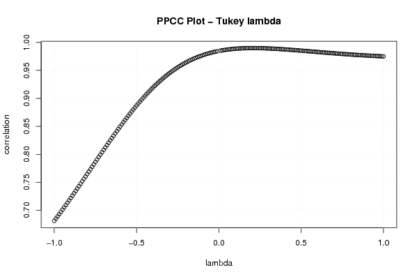
bitmap(file='test1.png')
plot((-100:100)/100,c[1:201],xlab='lambda',ylab='correlation',main='PPCC Plot - Tukey lambda')
grid()
dev.off()
load(file='createtable')
a<-table.start()
a<-table.row.start(a)
a<-table.element(a,'Tukey Lambda - Key Values',2,TRUE)
a<-table.row.end(a)
a<-table.row.start(a)
a<-table.element(a,'Distribution (lambda)',1,TRUE)
a<-table.element(a,'Correlation',1,TRUE)
a<-table.row.end(a)
a<-table.row.start(a)
a<-table.element(a,'Approx. Cauchy (lambda=-1)',header=TRUE)
a<-table.element(a,c[1])
a<-table.row.end(a)
a<-table.row.start(a)
a<-table.element(a,'Exact Logistic (lambda=0)',header=TRUE)
a<-table.element(a,(c[100]+c[102])/2)
a<-table.row.end(a)
a<-table.row.start(a)
a<-table.element(a,'Approx. Normal (lambda=0.14)',header=TRUE)
a<-table.element(a,c[115])
a<-table.row.end(a)
a<-table.row.start(a)
a<-table.element(a,'U-shaped (lambda=0.5)',header=TRUE)
a<-table.element(a,c[151])
a<-table.row.end(a)
a<-table.row.start(a)
a<-table.element(a,'Exactly Uniform (lambda=1)',header=TRUE)
a<-table.element(a,c[201])
a<-table.row.end(a)
a<-table.end(a)
table.save(a,file='mytable.tab')

Free Statistics

Description of Statistical Computation

Tree of Dependent Computations

Dataset

Tables (Output of Computation)

Figures (Output of Computation)

Input Parameters & R Code