Free Statistics
of Irreproducible Research!
Description of Statistical Computation | |||||||||||||||||||||||||||||||||||||||||||||||||||||
|---|---|---|---|---|---|---|---|---|---|---|---|---|---|---|---|---|---|---|---|---|---|---|---|---|---|---|---|---|---|---|---|---|---|---|---|---|---|---|---|---|---|---|---|---|---|---|---|---|---|---|---|---|---|
| Author's title | |||||||||||||||||||||||||||||||||||||||||||||||||||||
| Author | *The author of this computation has been verified* | ||||||||||||||||||||||||||||||||||||||||||||||||||||
| R Software Module | rwasp_edauni.wasp | ||||||||||||||||||||||||||||||||||||||||||||||||||||
| Title produced by software | Univariate Explorative Data Analysis | ||||||||||||||||||||||||||||||||||||||||||||||||||||
| Date of computation | Thu, 23 Oct 2008 06:34:55 -0600 | ||||||||||||||||||||||||||||||||||||||||||||||||||||
| Cite this page as follows | Statistical Computations at FreeStatistics.org, Office for Research Development and Education, URL https://freestatistics.org/blog/index.php?v=date/2008/Oct/23/t1224765382m92le54q41i8u02.htm/, Retrieved Sun, 19 May 2024 12:56:35 +0000 | ||||||||||||||||||||||||||||||||||||||||||||||||||||
| Statistical Computations at FreeStatistics.org, Office for Research Development and Education, URL https://freestatistics.org/blog/index.php?pk=18491, Retrieved Sun, 19 May 2024 12:56:35 +0000 | |||||||||||||||||||||||||||||||||||||||||||||||||||||
| QR Codes: | |||||||||||||||||||||||||||||||||||||||||||||||||||||
|
| |||||||||||||||||||||||||||||||||||||||||||||||||||||
| Original text written by user: | |||||||||||||||||||||||||||||||||||||||||||||||||||||
| IsPrivate? | No (this computation is public) | ||||||||||||||||||||||||||||||||||||||||||||||||||||
| User-defined keywords | distribution Q2 | ||||||||||||||||||||||||||||||||||||||||||||||||||||
| Estimated Impact | 199 | ||||||||||||||||||||||||||||||||||||||||||||||||||||
Tree of Dependent Computations | |||||||||||||||||||||||||||||||||||||||||||||||||||||
| Family? (F = Feedback message, R = changed R code, M = changed R Module, P = changed Parameters, D = changed Data) | |||||||||||||||||||||||||||||||||||||||||||||||||||||
| F [Univariate Explorative Data Analysis] [Investigation Dis...] [2007-10-21 17:06:37] [b9964c45117f7aac638ab9056d451faa] F R D [Univariate Explorative Data Analysis] [univariate explor...] [2008-10-23 12:34:55] [3817f5e632a8bfeb1be7b5e8c86bd450] [Current] F D [Univariate Explorative Data Analysis] [Clothing/Total Pr...] [2008-10-23 13:17:47] [077ffec662d24c06be4c491541a44245] F [Univariate Explorative Data Analysis] [] [2008-10-25 13:20:42] [4c8dfb519edec2da3492d7e6be9a5685] - RMPD [] [confidence interv...] [-0001-11-30 00:00:00] [077ffec662d24c06be4c491541a44245] F RMPD [Harrell-Davis Quantiles] [Harrel davies met...] [2008-10-23 14:25:11] [077ffec662d24c06be4c491541a44245] F P [Harrell-Davis Quantiles] [] [2008-10-25 13:29:43] [4c8dfb519edec2da3492d7e6be9a5685] - R [Harrell-Davis Quantiles] [Distribution verb...] [2008-10-28 17:04:37] [077ffec662d24c06be4c491541a44245] F RM D [Central Tendency] [mean of the error] [2008-10-23 14:45:08] [077ffec662d24c06be4c491541a44245] F [Central Tendency] [] [2008-10-25 13:55:42] [4c8dfb519edec2da3492d7e6be9a5685] - [Univariate Explorative Data Analysis] [] [2008-10-25 13:05:09] [4c8dfb519edec2da3492d7e6be9a5685] F [Univariate Explorative Data Analysis] [] [2008-10-25 13:08:49] [4c8dfb519edec2da3492d7e6be9a5685] F P [Univariate Explorative Data Analysis] [] [2008-10-25 14:19:35] [4c8dfb519edec2da3492d7e6be9a5685] F P [Univariate Explorative Data Analysis] [] [2008-10-25 14:25:52] [4c8dfb519edec2da3492d7e6be9a5685] F [Univariate Explorative Data Analysis] [] [2008-10-27 08:04:13] [077ffec662d24c06be4c491541a44245] F [Univariate Explorative Data Analysis] [] [2008-10-27 08:02:47] [077ffec662d24c06be4c491541a44245] - P [Univariate Explorative Data Analysis] [Verbetering distr...] [2008-10-28 15:34:23] [077ffec662d24c06be4c491541a44245] - RMP [Central Tendency] [distribution verb...] [2008-10-28 16:04:07] [077ffec662d24c06be4c491541a44245] - P [Univariate Explorative Data Analysis] [] [2008-11-03 11:22:47] [2a0ad3a9bcadca2da0acb91636601c6c] | |||||||||||||||||||||||||||||||||||||||||||||||||||||
| Feedback Forum | |||||||||||||||||||||||||||||||||||||||||||||||||||||
Post a new message | |||||||||||||||||||||||||||||||||||||||||||||||||||||
Dataset | |||||||||||||||||||||||||||||||||||||||||||||||||||||
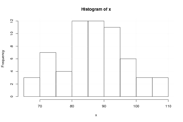
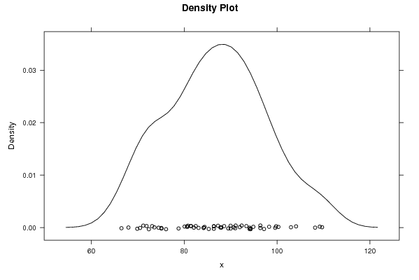
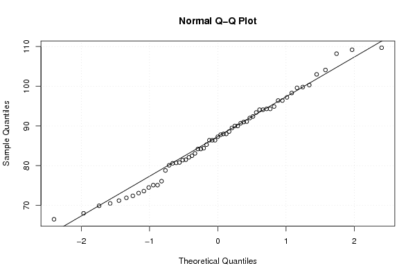
| Dataseries X: | |||||||||||||||||||||||||||||||||||||||||||||||||||||
109.20 88.60 94.30 98.30 86.40 80.60 104.10 108.20 93.40 71.90 94.10 94.90 96.40 91.10 84.40 86.40 88.00 75.10 109.70 103.00 82.10 68.00 96.40 94.30 90.00 88.00 76.10 82.50 81.40 66.50 97.20 94.10 80.70 70.50 87.80 89.50 99.60 84.20 75.10 92.00 80.80 73.10 99.80 90.00 83.10 72.40 78.80 87.30 91.00 80.10 73.60 86.40 74.50 71.20 92.40 81.50 85.30 69.90 84.20 90.70 100.30 | |||||||||||||||||||||||||||||||||||||||||||||||||||||
Tables (Output of Computation) | |||||||||||||||||||||||||||||||||||||||||||||||||||||
| |||||||||||||||||||||||||||||||||||||||||||||||||||||
Figures (Output of Computation) | |||||||||||||||||||||||||||||||||||||||||||||||||||||
Input Parameters & R Code | |||||||||||||||||||||||||||||||||||||||||||||||||||||
| Parameters (Session): | |||||||||||||||||||||||||||||||||||||||||||||||||||||
| par1 = 0 ; par2 = 0 ; | |||||||||||||||||||||||||||||||||||||||||||||||||||||
| Parameters (R input): | |||||||||||||||||||||||||||||||||||||||||||||||||||||
| par1 = 0 ; par2 = 0 ; | |||||||||||||||||||||||||||||||||||||||||||||||||||||
| R code (references can be found in the software module): | |||||||||||||||||||||||||||||||||||||||||||||||||||||
par1 <- as.numeric(par1) | |||||||||||||||||||||||||||||||||||||||||||||||||||||