Free Statistics
of Irreproducible Research!
Description of Statistical Computation | |||||||||||||||||||||||||||||||||||||||||||||||||||||
|---|---|---|---|---|---|---|---|---|---|---|---|---|---|---|---|---|---|---|---|---|---|---|---|---|---|---|---|---|---|---|---|---|---|---|---|---|---|---|---|---|---|---|---|---|---|---|---|---|---|---|---|---|---|
| Author's title | |||||||||||||||||||||||||||||||||||||||||||||||||||||
| Author | *The author of this computation has been verified* | ||||||||||||||||||||||||||||||||||||||||||||||||||||
| R Software Module | rwasp_edauni.wasp | ||||||||||||||||||||||||||||||||||||||||||||||||||||
| Title produced by software | Univariate Explorative Data Analysis | ||||||||||||||||||||||||||||||||||||||||||||||||||||
| Date of computation | Thu, 23 Oct 2008 06:24:03 -0600 | ||||||||||||||||||||||||||||||||||||||||||||||||||||
| Cite this page as follows | Statistical Computations at FreeStatistics.org, Office for Research Development and Education, URL https://freestatistics.org/blog/index.php?v=date/2008/Oct/23/t1224764711fqxt1dpnpzyc2e4.htm/, Retrieved Sun, 19 May 2024 14:38:48 +0000 | ||||||||||||||||||||||||||||||||||||||||||||||||||||
| Statistical Computations at FreeStatistics.org, Office for Research Development and Education, URL https://freestatistics.org/blog/index.php?pk=18487, Retrieved Sun, 19 May 2024 14:38:48 +0000 | |||||||||||||||||||||||||||||||||||||||||||||||||||||
| QR Codes: | |||||||||||||||||||||||||||||||||||||||||||||||||||||
|
| |||||||||||||||||||||||||||||||||||||||||||||||||||||
| Original text written by user: | |||||||||||||||||||||||||||||||||||||||||||||||||||||
| IsPrivate? | No (this computation is public) | ||||||||||||||||||||||||||||||||||||||||||||||||||||
| User-defined keywords | |||||||||||||||||||||||||||||||||||||||||||||||||||||
| Estimated Impact | 242 | ||||||||||||||||||||||||||||||||||||||||||||||||||||
Tree of Dependent Computations | |||||||||||||||||||||||||||||||||||||||||||||||||||||
| Family? (F = Feedback message, R = changed R code, M = changed R Module, P = changed Parameters, D = changed Data) | |||||||||||||||||||||||||||||||||||||||||||||||||||||
| F [Univariate Explorative Data Analysis] [Q2 kledij] [2008-10-23 12:24:03] [b23db733701c4d62df5e228d507c1c6a] [Current] F R [Univariate Explorative Data Analysis] [Q2 Investigating ...] [2008-10-24 17:21:50] [29647dffafb5b58c12a48dbf6cba2b57] F [Univariate Explorative Data Analysis] [Univariate explor...] [2008-10-27 09:05:47] [b5373f20234c18c6452d5f98d8abf0fe] - RMP [Central Tendency] [Q2 verbetering] [2008-10-28 18:57:50] [46c5a5fbda57fdfa1d4ef48658f82a0c] - R [Central Tendency] [Q2 verbetering (2)] [2008-10-28 19:00:48] [46c5a5fbda57fdfa1d4ef48658f82a0c] - D [Univariate Explorative Data Analysis] [Investigating Dis...] [2008-12-19 20:31:13] [29647dffafb5b58c12a48dbf6cba2b57] - [Univariate Explorative Data Analysis] [Investigating Dis...] [2008-12-20 16:04:20] [70cb582895831af4be81fec73c607e93] - RMPD [Notched Boxplots] [Evelyn] [2008-12-20 16:07:43] [29647dffafb5b58c12a48dbf6cba2b57] | |||||||||||||||||||||||||||||||||||||||||||||||||||||
| Feedback Forum | |||||||||||||||||||||||||||||||||||||||||||||||||||||
Post a new message | |||||||||||||||||||||||||||||||||||||||||||||||||||||
Dataset | |||||||||||||||||||||||||||||||||||||||||||||||||||||
| Dataseries X: | |||||||||||||||||||||||||||||||||||||||||||||||||||||
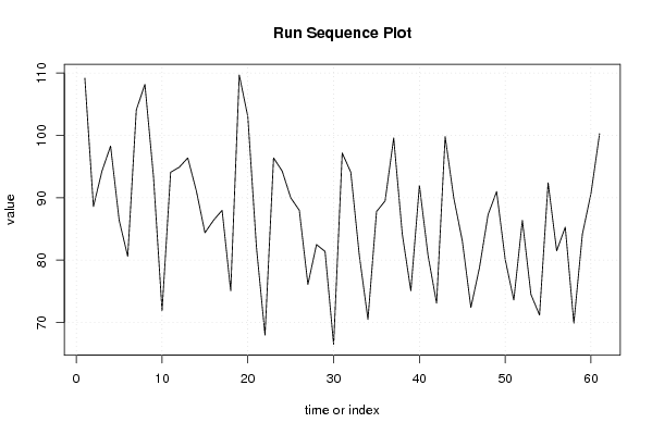
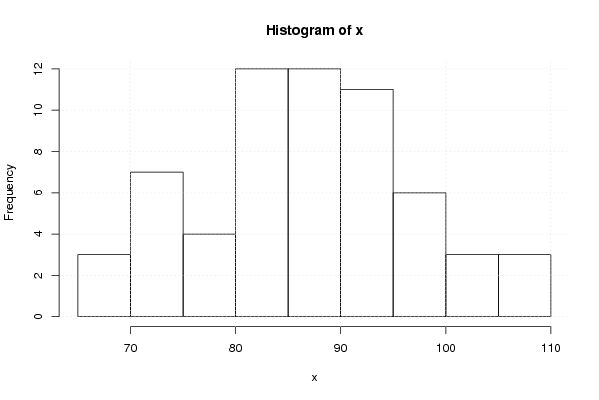
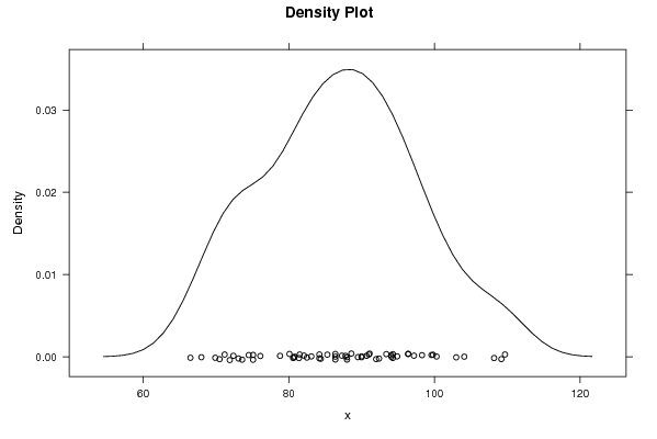
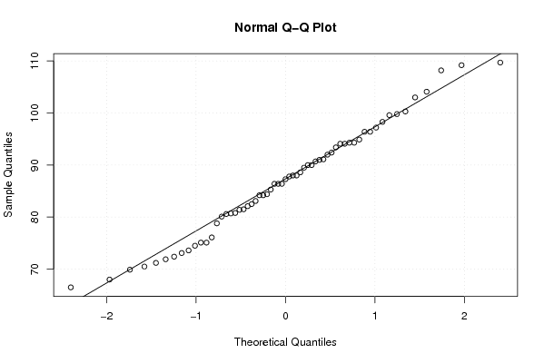
109.20 88.60 94.30 98.30 86.40 80.60 104.10 108.20 93.40 71.90 94.10 94.90 96.40 91.10 84.40 86.40 88.00 75.10 109.70 103.00 82.10 68.00 96.40 94.30 90.00 88.00 76.10 82.50 81.40 66.50 97.20 94.10 80.70 70.50 87.80 89.50 99.60 84.20 75.10 92.00 80.80 73.10 99.80 90.00 83.10 72.40 78.80 87.30 91.00 80.10 73.60 86.40 74.50 71.20 92.40 81.50 85.30 69.90 84.20 90.70 100.30 | |||||||||||||||||||||||||||||||||||||||||||||||||||||
Tables (Output of Computation) | |||||||||||||||||||||||||||||||||||||||||||||||||||||
| |||||||||||||||||||||||||||||||||||||||||||||||||||||
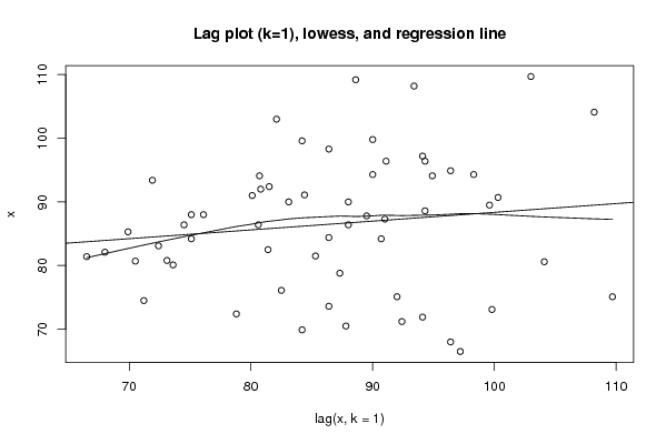
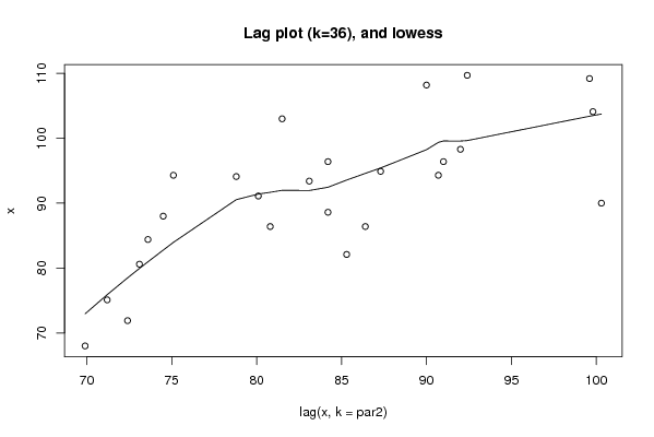
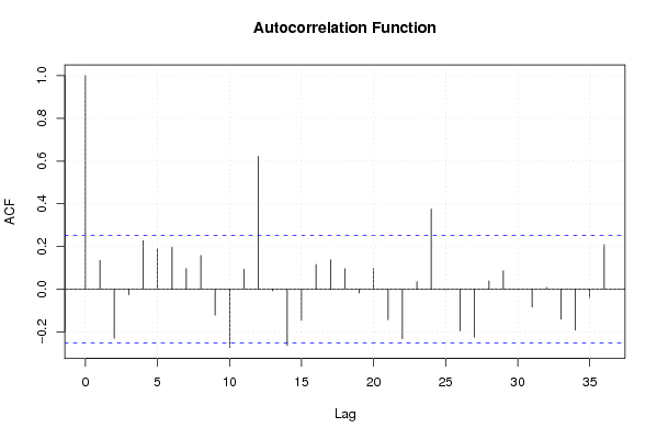
Figures (Output of Computation) | |||||||||||||||||||||||||||||||||||||||||||||||||||||
Input Parameters & R Code | |||||||||||||||||||||||||||||||||||||||||||||||||||||
| Parameters (Session): | |||||||||||||||||||||||||||||||||||||||||||||||||||||
| par1 = 0 ; par2 = 36 ; | |||||||||||||||||||||||||||||||||||||||||||||||||||||
| Parameters (R input): | |||||||||||||||||||||||||||||||||||||||||||||||||||||
| par1 = 0 ; par2 = 36 ; | |||||||||||||||||||||||||||||||||||||||||||||||||||||
| R code (references can be found in the software module): | |||||||||||||||||||||||||||||||||||||||||||||||||||||
par1 <- as.numeric(par1) | |||||||||||||||||||||||||||||||||||||||||||||||||||||