Free Statistics
of Irreproducible Research!
Description of Statistical Computation | |||||||||||||||||||||
|---|---|---|---|---|---|---|---|---|---|---|---|---|---|---|---|---|---|---|---|---|---|
| Author's title | |||||||||||||||||||||
| Author | *The author of this computation has been verified* | ||||||||||||||||||||
| R Software Module | rwasp_backtobackhist.wasp | ||||||||||||||||||||
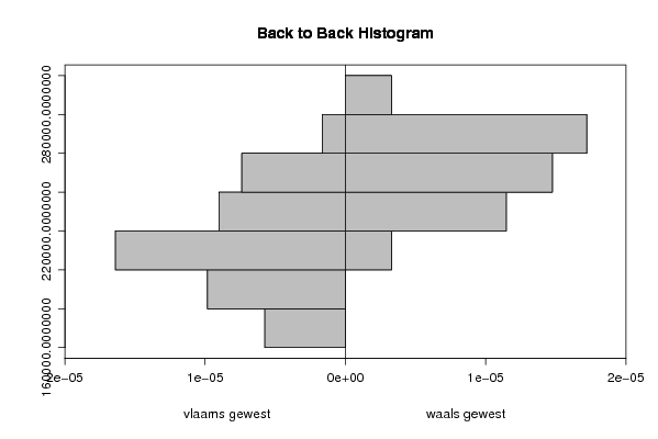
| Title produced by software | Back to Back Histogram | ||||||||||||||||||||
| Date of computation | Mon, 20 Oct 2008 10:51:01 -0600 | ||||||||||||||||||||
| Cite this page as follows | Statistical Computations at FreeStatistics.org, Office for Research Development and Education, URL https://freestatistics.org/blog/index.php?v=date/2008/Oct/20/t122452152085ijh3ddi77c528.htm/, Retrieved Sun, 19 May 2024 15:53:37 +0000 | ||||||||||||||||||||
| Statistical Computations at FreeStatistics.org, Office for Research Development and Education, URL https://freestatistics.org/blog/index.php?pk=17641, Retrieved Sun, 19 May 2024 15:53:37 +0000 | |||||||||||||||||||||
| QR Codes: | |||||||||||||||||||||
|
| |||||||||||||||||||||
| Original text written by user: | |||||||||||||||||||||
| IsPrivate? | No (this computation is public) | ||||||||||||||||||||
| User-defined keywords | |||||||||||||||||||||
| Estimated Impact | 100 | ||||||||||||||||||||
Tree of Dependent Computations | |||||||||||||||||||||
| Family? (F = Feedback message, R = changed R code, M = changed R Module, P = changed Parameters, D = changed Data) | |||||||||||||||||||||
| F [Back to Back Histogram] [Back to back hist...] [2008-10-20 16:51:01] [bda7fba231d49184c6a1b627868bbb81] [Current] | |||||||||||||||||||||
| Feedback Forum | |||||||||||||||||||||
Post a new message | |||||||||||||||||||||
Dataset | |||||||||||||||||||||
| Dataseries X: | |||||||||||||||||||||
189917 184128 175335 179566 181140 177876 175041 169292 166070 166972 206348 215706 202108 195411 193111 195198 198770 194163 190420 189733 186029 191531 232571 243477 227247 217859 208679 213188 216234 213587 209465 204045 200237 203666 241476 260307 243324 244460 233575 237217 235243 230354 227184 221678 217142 219452 256446 265845 248624 241114 229245 231805 219277 219313 212610 214771 211142 211457 240048 240636 230580 | |||||||||||||||||||||
| Dataseries Y: | |||||||||||||||||||||
250853 245775 220309 216689 220316 220726 220286 216507 213020 213001 231854 236386 241168 240326 234294 235304 238127 238726 235694 236660 232986 233705 253525 254303 261224 258778 252791 256389 258961 258647 256304 250498 247883 249552 262626 264416 273049 272441 267564 265952 263937 264765 263386 258985 257334 257477 271486 274488 281274 272674 269704 268227 276444 272247 268516 263406 263619 265905 281681 287413 289423 | |||||||||||||||||||||
Tables (Output of Computation) | |||||||||||||||||||||
| |||||||||||||||||||||
Figures (Output of Computation) | |||||||||||||||||||||
Input Parameters & R Code | |||||||||||||||||||||
| Parameters (Session): | |||||||||||||||||||||
| par1 = grey ; par2 = grey ; par3 = TRUE ; par4 = vlaams gewest ; par5 = waals gewest ; | |||||||||||||||||||||
| Parameters (R input): | |||||||||||||||||||||
| par1 = grey ; par2 = grey ; par3 = TRUE ; par4 = vlaams gewest ; par5 = waals gewest ; | |||||||||||||||||||||
| R code (references can be found in the software module): | |||||||||||||||||||||
if (par3 == 'TRUE') par3 <- TRUE | |||||||||||||||||||||