Repository of Reproducible Computations

Free Statistics

of Irreproducible Research!

Author's title

Author

*The author of this computation has been verified*

R Software Module

rwasp_percentiles.wasp

Title produced by software

Percentiles

Date of computation

Mon, 20 Oct 2008 09:03:31 -0600

Cite this page as follows

Statistical Computations at FreeStatistics.org, Office for Research Development and Education, URL https://freestatistics.org/blog/index.php?v=date/2008/Oct/20/t1224515049ik6lcssl83cysno.htm/, Retrieved Sun, 19 May 2024 13:21:19 +0000

Statistical Computations at FreeStatistics.org, Office for Research Development and Education, URL https://freestatistics.org/blog/index.php?pk=17423, Retrieved Sun, 19 May 2024 13:21:19 +0000

QR Codes:

Paste this QR Code to cite your computation.

Original text written by user:

IsPrivate?

No (this computation is public)

User-defined keywords

percentiles prijzen uitvoer

Estimated Impact

151

Family? (F = Feedback message, R = changed R code, M = changed R Module, P = changed Parameters, D = changed Data)

-     [Central Tendency] [Central Tendency:...] [2008-10-20 13:43:11] [9e54d1454d464f1bf9ee4a54d5d56945]
-    D  [Central Tendency] [Central Tendency ...] [2008-10-20 13:47:13] [9e54d1454d464f1bf9ee4a54d5d56945]
- RMPD      [Percentiles] [Percentiles Prijz...] [2008-10-20 15:03:31] [8da7502cfecb272886bc60b3f290b8b8] [Current]
-    D        [Percentiles] [Percentiles Wisse...] [2008-10-20 15:06:01] [9e54d1454d464f1bf9ee4a54d5d56945] 
- RM D        [Back to Back Histogram] [Back bo back hist...] [2008-10-20 15:18:42] [9e54d1454d464f1bf9ee4a54d5d56945] 
- RM D        [Back to Back Histogram] [Back to back hist...] [2008-10-20 15:21:15] [9e54d1454d464f1bf9ee4a54d5d56945] 
- RM D        [Central Tendency] [Central tendency ...] [2008-10-20 17:18:05] [9e54d1454d464f1bf9ee4a54d5d56945] 
F RM D        [Central Tendency] [Central tendency ...] [2008-10-20 17:20:48] [9e54d1454d464f1bf9ee4a54d5d56945] 
-   P           [Central Tendency] [Central Tendency ...] [2008-10-20 21:47:27] [706ea9a318c13a45c936b5008831fe13] 
- RM D        [Central Tendency] [Central tendency ...] [2008-10-20 17:23:39] [9e54d1454d464f1bf9ee4a54d5d56945] 
F RM D        [Central Tendency] [Central tendency ...] [2008-10-20 17:27:05] [9e54d1454d464f1bf9ee4a54d5d56945] 

Feedback Forum

Post a new message

Dataseries X:

Download CSV

Histogram

Boxplots

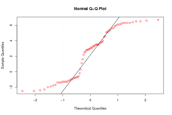
-1,3
-1,4
-1,3
-1
-0,8
-0,7
-0,6
-0,8
-0,9
-1
-1,2
-1,3
-1,3
-1,4
-1,4
-1,8
-1,9
-2
-2,4
-2,5
-2,5
-2,3
-1,7
-1,1
-0,7
-0,2
0,3
1,1
1,6
2,2
3
3,8
4,6
5,1
5,3
5,5
5,7
5,9
6,1
6,1
6,3
6,5
6,7
6,6
6,5
6,4
6,3
6,3
6,3
6,2
6
5,6
5,3
5,1
4,5
4
3,5
3,5
3,3
3,1
2,9
2,5
2,6
2,8
2,8
2,9
3,1
3,3
3,5
3,4
3,5
3,7
3,8

Summary of computational transaction
Raw Input	view raw input (R code)
Raw Output	view raw output of R engine
Computing time	1 seconds
R Server	'George Udny Yule' @ 72.249.76.132

\begin{tabular}{lllllllll}
\hline
Summary of computational transaction \tabularnewline
Raw Input & view raw input (R code)  \tabularnewline
Raw Output & view raw output of R engine  \tabularnewline
Computing time & 1 seconds \tabularnewline
R Server & 'George Udny Yule' @ 72.249.76.132 \tabularnewline
\hline
\end{tabular}
%Source: https://freestatistics.org/blog/index.php?pk=17423&T=0

[TABLE]
[ROW][C]Summary of computational transaction[/C][/ROW]
[ROW][C]Raw Input[/C][C]view raw input (R code) [/C][/ROW]
[ROW][C]Raw Output[/C][C]view raw output of R engine [/C][/ROW]
[ROW][C]Computing time[/C][C]1 seconds[/C][/ROW]
[ROW][C]R Server[/C][C]'George Udny Yule' @ 72.249.76.132[/C][/ROW]
[/TABLE]
Source: https://freestatistics.org/blog/index.php?pk=17423&T=0

Globally Unique Identifier (entire table): ba.freestatistics.org/blog/index.php?pk=17423&T=0

As an alternative you can also use a QR Code:

The GUIDs for individual cells are displayed in the table below:

Summary of computational transaction
Raw Input	view raw input (R code)
Raw Output	view raw output of R engine
Computing time	1 seconds
R Server	'George Udny Yule' @ 72.249.76.132

Percentiles - Ungrouped Data
p	Weighted Average at Xnp	Weighted Average at X(n+1)p	Empirical Distribution Function	Empirical Distribution Function - Averaging	Empirical Distribution Function - Interpolation	Closest Observation	True Basic - Statistics Graphics Toolkit	MS Excel (old versions)
0.02	-2.5	-2.5	-2.5	-2.5	-2.456	-2.5	-2.5	-2.5
0.04	-2.408	-2.404	-2.4	-2.4	-2.312	-2.4	-2.496	-2.4
0.06	-2.186	-2.168	-2	-2	-1.968	-2.3	-2.132	-2.3
0.08	-1.916	-1.908	-1.9	-1.9	-1.824	-1.9	-1.992	-1.9
0.1	-1.77	-1.76	-1.7	-1.7	-1.64	-1.8	-1.74	-1.8
0.12	-1.472	-1.436	-1.4	-1.4	-1.4	-1.4	-1.664	-1.4
0.14	-1.4	-1.4	-1.4	-1.4	-1.392	-1.4	-1.4	-1.4
0.16	-1.332	-1.316	-1.3	-1.3	-1.3	-1.3	-1.384	-1.3
0.18	-1.3	-1.3	-1.3	-1.3	-1.3	-1.3	-1.3	-1.3
0.2	-1.3	-1.3	-1.3	-1.3	-1.26	-1.3	-1.3	-1.3
0.22	-1.194	-1.172	-1.1	-1.1	-1.116	-1.2	-1.128	-1.2
0.24	-1.048	-1.024	-1	-1	-1	-1	-1.076	-1
0.26	-1	-0.976	-1	-1	-0.928	-1	-0.924	-1
0.28	-0.856	-0.828	-0.8	-0.8	-0.8	-0.9	-0.872	-0.8
0.3	-0.8	-0.78	-0.8	-0.8	-0.74	-0.8	-0.72	-0.8
0.32	-0.7	-0.7	-0.7	-0.7	-0.696	-0.7	-0.7	-0.7
0.34	-0.618	-0.536	-0.6	-0.6	-0.408	-0.6	-0.264	-0.6
0.36	-0.06	0.12	0.3	0.3	0.26	-0.2	-0.02	0.3
0.38	0.892	1.16	1.1	1.1	1.28	1.1	1.54	1.1
0.4	1.72	1.96	2.2	2.2	2.08	1.6	1.84	2.2
0.42	2.398	2.508	2.5	2.5	2.524	2.5	2.592	2.5
0.44	2.624	2.712	2.8	2.8	2.736	2.6	2.688	2.8
0.46	2.8	2.804	2.8	2.8	2.812	2.8	2.896	2.8
0.48	2.9	2.9	2.9	2.9	2.9	2.9	2.9	2.9
0.5	2.95	3	3	3	3	3	3	3
0.52	3.096	3.1	3.1	3.1	3.1	3.1	3.1	3.1
0.54	3.184	3.292	3.3	3.3	3.276	3.1	3.108	3.3
0.56	3.3	3.344	3.3	3.3	3.332	3.3	3.356	3.3
0.58	3.434	3.492	3.5	3.5	3.476	3.4	3.408	3.5
0.6	3.5	3.5	3.5	3.5	3.5	3.5	3.5	3.5
0.62	3.5	3.5	3.5	3.5	3.5	3.5	3.5	3.5
0.64	3.644	3.736	3.7	3.7	3.708	3.7	3.764	3.7
0.66	3.8	3.8	3.8	3.8	3.8	3.8	3.8	3.8
0.68	3.928	4.16	4	4	3.992	4	4.34	4
0.7	4.51	4.58	4.6	4.6	4.54	4.5	4.52	4.6
0.72	4.88	5.1	5.1	5.1	5.02	5.1	5.1	5.1
0.74	5.104	5.252	5.3	5.3	5.156	5.1	5.148	5.3
0.76	5.3	5.348	5.3	5.3	5.3	5.3	5.452	5.3
0.78	5.488	5.572	5.5	5.5	5.516	5.5	5.528	5.6
0.8	5.64	5.74	5.7	5.7	5.66	5.6	5.86	5.7
0.82	5.872	5.968	5.9	5.9	5.904	5.9	5.932	6
0.84	6.032	6.1	6.1	6.1	6.048	6	6.1	6.1
0.86	6.1	6.164	6.1	6.1	6.1	6.1	6.136	6.2
0.88	6.224	6.3	6.3	6.3	6.236	6.2	6.3	6.3
0.9	6.3	6.3	6.3	6.3	6.3	6.3	6.3	6.3
0.92	6.3	6.308	6.3	6.3	6.3	6.3	6.392	6.3
0.94	6.362	6.456	6.4	6.4	6.368	6.4	6.444	6.5
0.96	6.5	6.504	6.5	6.5	6.5	6.5	6.596	6.5
0.98	6.554	6.652	6.6	6.6	6.556	6.6	6.648	6.7

\begin{tabular}{lllllllll}
\hline
Percentiles - Ungrouped Data \tabularnewline
p & Weighted Average at Xnp & Weighted Average at X(n+1)p & Empirical Distribution Function & Empirical Distribution Function - Averaging & Empirical Distribution Function - Interpolation & Closest Observation & True Basic - Statistics Graphics Toolkit & MS Excel (old versions) \tabularnewline
0.02 & -2.5 & -2.5 & -2.5 & -2.5 & -2.456 & -2.5 & -2.5 & -2.5 \tabularnewline
0.04 & -2.408 & -2.404 & -2.4 & -2.4 & -2.312 & -2.4 & -2.496 & -2.4 \tabularnewline
0.06 & -2.186 & -2.168 & -2 & -2 & -1.968 & -2.3 & -2.132 & -2.3 \tabularnewline
0.08 & -1.916 & -1.908 & -1.9 & -1.9 & -1.824 & -1.9 & -1.992 & -1.9 \tabularnewline
0.1 & -1.77 & -1.76 & -1.7 & -1.7 & -1.64 & -1.8 & -1.74 & -1.8 \tabularnewline
0.12 & -1.472 & -1.436 & -1.4 & -1.4 & -1.4 & -1.4 & -1.664 & -1.4 \tabularnewline
0.14 & -1.4 & -1.4 & -1.4 & -1.4 & -1.392 & -1.4 & -1.4 & -1.4 \tabularnewline
0.16 & -1.332 & -1.316 & -1.3 & -1.3 & -1.3 & -1.3 & -1.384 & -1.3 \tabularnewline
0.18 & -1.3 & -1.3 & -1.3 & -1.3 & -1.3 & -1.3 & -1.3 & -1.3 \tabularnewline
0.2 & -1.3 & -1.3 & -1.3 & -1.3 & -1.26 & -1.3 & -1.3 & -1.3 \tabularnewline
0.22 & -1.194 & -1.172 & -1.1 & -1.1 & -1.116 & -1.2 & -1.128 & -1.2 \tabularnewline
0.24 & -1.048 & -1.024 & -1 & -1 & -1 & -1 & -1.076 & -1 \tabularnewline
0.26 & -1 & -0.976 & -1 & -1 & -0.928 & -1 & -0.924 & -1 \tabularnewline
0.28 & -0.856 & -0.828 & -0.8 & -0.8 & -0.8 & -0.9 & -0.872 & -0.8 \tabularnewline
0.3 & -0.8 & -0.78 & -0.8 & -0.8 & -0.74 & -0.8 & -0.72 & -0.8 \tabularnewline
0.32 & -0.7 & -0.7 & -0.7 & -0.7 & -0.696 & -0.7 & -0.7 & -0.7 \tabularnewline
0.34 & -0.618 & -0.536 & -0.6 & -0.6 & -0.408 & -0.6 & -0.264 & -0.6 \tabularnewline
0.36 & -0.06 & 0.12 & 0.3 & 0.3 & 0.26 & -0.2 & -0.02 & 0.3 \tabularnewline
0.38 & 0.892 & 1.16 & 1.1 & 1.1 & 1.28 & 1.1 & 1.54 & 1.1 \tabularnewline
0.4 & 1.72 & 1.96 & 2.2 & 2.2 & 2.08 & 1.6 & 1.84 & 2.2 \tabularnewline
0.42 & 2.398 & 2.508 & 2.5 & 2.5 & 2.524 & 2.5 & 2.592 & 2.5 \tabularnewline
0.44 & 2.624 & 2.712 & 2.8 & 2.8 & 2.736 & 2.6 & 2.688 & 2.8 \tabularnewline
0.46 & 2.8 & 2.804 & 2.8 & 2.8 & 2.812 & 2.8 & 2.896 & 2.8 \tabularnewline
0.48 & 2.9 & 2.9 & 2.9 & 2.9 & 2.9 & 2.9 & 2.9 & 2.9 \tabularnewline
0.5 & 2.95 & 3 & 3 & 3 & 3 & 3 & 3 & 3 \tabularnewline
0.52 & 3.096 & 3.1 & 3.1 & 3.1 & 3.1 & 3.1 & 3.1 & 3.1 \tabularnewline
0.54 & 3.184 & 3.292 & 3.3 & 3.3 & 3.276 & 3.1 & 3.108 & 3.3 \tabularnewline
0.56 & 3.3 & 3.344 & 3.3 & 3.3 & 3.332 & 3.3 & 3.356 & 3.3 \tabularnewline
0.58 & 3.434 & 3.492 & 3.5 & 3.5 & 3.476 & 3.4 & 3.408 & 3.5 \tabularnewline
0.6 & 3.5 & 3.5 & 3.5 & 3.5 & 3.5 & 3.5 & 3.5 & 3.5 \tabularnewline
0.62 & 3.5 & 3.5 & 3.5 & 3.5 & 3.5 & 3.5 & 3.5 & 3.5 \tabularnewline
0.64 & 3.644 & 3.736 & 3.7 & 3.7 & 3.708 & 3.7 & 3.764 & 3.7 \tabularnewline
0.66 & 3.8 & 3.8 & 3.8 & 3.8 & 3.8 & 3.8 & 3.8 & 3.8 \tabularnewline
0.68 & 3.928 & 4.16 & 4 & 4 & 3.992 & 4 & 4.34 & 4 \tabularnewline
0.7 & 4.51 & 4.58 & 4.6 & 4.6 & 4.54 & 4.5 & 4.52 & 4.6 \tabularnewline
0.72 & 4.88 & 5.1 & 5.1 & 5.1 & 5.02 & 5.1 & 5.1 & 5.1 \tabularnewline
0.74 & 5.104 & 5.252 & 5.3 & 5.3 & 5.156 & 5.1 & 5.148 & 5.3 \tabularnewline
0.76 & 5.3 & 5.348 & 5.3 & 5.3 & 5.3 & 5.3 & 5.452 & 5.3 \tabularnewline
0.78 & 5.488 & 5.572 & 5.5 & 5.5 & 5.516 & 5.5 & 5.528 & 5.6 \tabularnewline
0.8 & 5.64 & 5.74 & 5.7 & 5.7 & 5.66 & 5.6 & 5.86 & 5.7 \tabularnewline
0.82 & 5.872 & 5.968 & 5.9 & 5.9 & 5.904 & 5.9 & 5.932 & 6 \tabularnewline
0.84 & 6.032 & 6.1 & 6.1 & 6.1 & 6.048 & 6 & 6.1 & 6.1 \tabularnewline
0.86 & 6.1 & 6.164 & 6.1 & 6.1 & 6.1 & 6.1 & 6.136 & 6.2 \tabularnewline
0.88 & 6.224 & 6.3 & 6.3 & 6.3 & 6.236 & 6.2 & 6.3 & 6.3 \tabularnewline
0.9 & 6.3 & 6.3 & 6.3 & 6.3 & 6.3 & 6.3 & 6.3 & 6.3 \tabularnewline
0.92 & 6.3 & 6.308 & 6.3 & 6.3 & 6.3 & 6.3 & 6.392 & 6.3 \tabularnewline
0.94 & 6.362 & 6.456 & 6.4 & 6.4 & 6.368 & 6.4 & 6.444 & 6.5 \tabularnewline
0.96 & 6.5 & 6.504 & 6.5 & 6.5 & 6.5 & 6.5 & 6.596 & 6.5 \tabularnewline
0.98 & 6.554 & 6.652 & 6.6 & 6.6 & 6.556 & 6.6 & 6.648 & 6.7 \tabularnewline
\hline
\end{tabular}
%Source: https://freestatistics.org/blog/index.php?pk=17423&T=1

[TABLE]
[ROW][C]Percentiles - Ungrouped Data[/C][/ROW]
[ROW][C]p[/C][C]Weighted Average at Xnp[/C][C]Weighted Average at X(n+1)p[/C][C]Empirical Distribution Function[/C][C]Empirical Distribution Function - Averaging[/C][C]Empirical Distribution Function - Interpolation[/C][C]Closest Observation[/C][C]True Basic - Statistics Graphics Toolkit[/C][C]MS Excel (old versions)[/C][/ROW]
[ROW][C]0.02[/C][C]-2.5[/C][C]-2.5[/C][C]-2.5[/C][C]-2.5[/C][C]-2.456[/C][C]-2.5[/C][C]-2.5[/C][C]-2.5[/C][/ROW]
[ROW][C]0.04[/C][C]-2.408[/C][C]-2.404[/C][C]-2.4[/C][C]-2.4[/C][C]-2.312[/C][C]-2.4[/C][C]-2.496[/C][C]-2.4[/C][/ROW]
[ROW][C]0.06[/C][C]-2.186[/C][C]-2.168[/C][C]-2[/C][C]-2[/C][C]-1.968[/C][C]-2.3[/C][C]-2.132[/C][C]-2.3[/C][/ROW]
[ROW][C]0.08[/C][C]-1.916[/C][C]-1.908[/C][C]-1.9[/C][C]-1.9[/C][C]-1.824[/C][C]-1.9[/C][C]-1.992[/C][C]-1.9[/C][/ROW]
[ROW][C]0.1[/C][C]-1.77[/C][C]-1.76[/C][C]-1.7[/C][C]-1.7[/C][C]-1.64[/C][C]-1.8[/C][C]-1.74[/C][C]-1.8[/C][/ROW]
[ROW][C]0.12[/C][C]-1.472[/C][C]-1.436[/C][C]-1.4[/C][C]-1.4[/C][C]-1.4[/C][C]-1.4[/C][C]-1.664[/C][C]-1.4[/C][/ROW]
[ROW][C]0.14[/C][C]-1.4[/C][C]-1.4[/C][C]-1.4[/C][C]-1.4[/C][C]-1.392[/C][C]-1.4[/C][C]-1.4[/C][C]-1.4[/C][/ROW]
[ROW][C]0.16[/C][C]-1.332[/C][C]-1.316[/C][C]-1.3[/C][C]-1.3[/C][C]-1.3[/C][C]-1.3[/C][C]-1.384[/C][C]-1.3[/C][/ROW]
[ROW][C]0.18[/C][C]-1.3[/C][C]-1.3[/C][C]-1.3[/C][C]-1.3[/C][C]-1.3[/C][C]-1.3[/C][C]-1.3[/C][C]-1.3[/C][/ROW]
[ROW][C]0.2[/C][C]-1.3[/C][C]-1.3[/C][C]-1.3[/C][C]-1.3[/C][C]-1.26[/C][C]-1.3[/C][C]-1.3[/C][C]-1.3[/C][/ROW]
[ROW][C]0.22[/C][C]-1.194[/C][C]-1.172[/C][C]-1.1[/C][C]-1.1[/C][C]-1.116[/C][C]-1.2[/C][C]-1.128[/C][C]-1.2[/C][/ROW]
[ROW][C]0.24[/C][C]-1.048[/C][C]-1.024[/C][C]-1[/C][C]-1[/C][C]-1[/C][C]-1[/C][C]-1.076[/C][C]-1[/C][/ROW]
[ROW][C]0.26[/C][C]-1[/C][C]-0.976[/C][C]-1[/C][C]-1[/C][C]-0.928[/C][C]-1[/C][C]-0.924[/C][C]-1[/C][/ROW]
[ROW][C]0.28[/C][C]-0.856[/C][C]-0.828[/C][C]-0.8[/C][C]-0.8[/C][C]-0.8[/C][C]-0.9[/C][C]-0.872[/C][C]-0.8[/C][/ROW]
[ROW][C]0.3[/C][C]-0.8[/C][C]-0.78[/C][C]-0.8[/C][C]-0.8[/C][C]-0.74[/C][C]-0.8[/C][C]-0.72[/C][C]-0.8[/C][/ROW]
[ROW][C]0.32[/C][C]-0.7[/C][C]-0.7[/C][C]-0.7[/C][C]-0.7[/C][C]-0.696[/C][C]-0.7[/C][C]-0.7[/C][C]-0.7[/C][/ROW]
[ROW][C]0.34[/C][C]-0.618[/C][C]-0.536[/C][C]-0.6[/C][C]-0.6[/C][C]-0.408[/C][C]-0.6[/C][C]-0.264[/C][C]-0.6[/C][/ROW]
[ROW][C]0.36[/C][C]-0.06[/C][C]0.12[/C][C]0.3[/C][C]0.3[/C][C]0.26[/C][C]-0.2[/C][C]-0.02[/C][C]0.3[/C][/ROW]
[ROW][C]0.38[/C][C]0.892[/C][C]1.16[/C][C]1.1[/C][C]1.1[/C][C]1.28[/C][C]1.1[/C][C]1.54[/C][C]1.1[/C][/ROW]
[ROW][C]0.4[/C][C]1.72[/C][C]1.96[/C][C]2.2[/C][C]2.2[/C][C]2.08[/C][C]1.6[/C][C]1.84[/C][C]2.2[/C][/ROW]
[ROW][C]0.42[/C][C]2.398[/C][C]2.508[/C][C]2.5[/C][C]2.5[/C][C]2.524[/C][C]2.5[/C][C]2.592[/C][C]2.5[/C][/ROW]
[ROW][C]0.44[/C][C]2.624[/C][C]2.712[/C][C]2.8[/C][C]2.8[/C][C]2.736[/C][C]2.6[/C][C]2.688[/C][C]2.8[/C][/ROW]
[ROW][C]0.46[/C][C]2.8[/C][C]2.804[/C][C]2.8[/C][C]2.8[/C][C]2.812[/C][C]2.8[/C][C]2.896[/C][C]2.8[/C][/ROW]
[ROW][C]0.48[/C][C]2.9[/C][C]2.9[/C][C]2.9[/C][C]2.9[/C][C]2.9[/C][C]2.9[/C][C]2.9[/C][C]2.9[/C][/ROW]
[ROW][C]0.5[/C][C]2.95[/C][C]3[/C][C]3[/C][C]3[/C][C]3[/C][C]3[/C][C]3[/C][C]3[/C][/ROW]
[ROW][C]0.52[/C][C]3.096[/C][C]3.1[/C][C]3.1[/C][C]3.1[/C][C]3.1[/C][C]3.1[/C][C]3.1[/C][C]3.1[/C][/ROW]
[ROW][C]0.54[/C][C]3.184[/C][C]3.292[/C][C]3.3[/C][C]3.3[/C][C]3.276[/C][C]3.1[/C][C]3.108[/C][C]3.3[/C][/ROW]
[ROW][C]0.56[/C][C]3.3[/C][C]3.344[/C][C]3.3[/C][C]3.3[/C][C]3.332[/C][C]3.3[/C][C]3.356[/C][C]3.3[/C][/ROW]
[ROW][C]0.58[/C][C]3.434[/C][C]3.492[/C][C]3.5[/C][C]3.5[/C][C]3.476[/C][C]3.4[/C][C]3.408[/C][C]3.5[/C][/ROW]
[ROW][C]0.6[/C][C]3.5[/C][C]3.5[/C][C]3.5[/C][C]3.5[/C][C]3.5[/C][C]3.5[/C][C]3.5[/C][C]3.5[/C][/ROW]
[ROW][C]0.62[/C][C]3.5[/C][C]3.5[/C][C]3.5[/C][C]3.5[/C][C]3.5[/C][C]3.5[/C][C]3.5[/C][C]3.5[/C][/ROW]
[ROW][C]0.64[/C][C]3.644[/C][C]3.736[/C][C]3.7[/C][C]3.7[/C][C]3.708[/C][C]3.7[/C][C]3.764[/C][C]3.7[/C][/ROW]
[ROW][C]0.66[/C][C]3.8[/C][C]3.8[/C][C]3.8[/C][C]3.8[/C][C]3.8[/C][C]3.8[/C][C]3.8[/C][C]3.8[/C][/ROW]
[ROW][C]0.68[/C][C]3.928[/C][C]4.16[/C][C]4[/C][C]4[/C][C]3.992[/C][C]4[/C][C]4.34[/C][C]4[/C][/ROW]
[ROW][C]0.7[/C][C]4.51[/C][C]4.58[/C][C]4.6[/C][C]4.6[/C][C]4.54[/C][C]4.5[/C][C]4.52[/C][C]4.6[/C][/ROW]
[ROW][C]0.72[/C][C]4.88[/C][C]5.1[/C][C]5.1[/C][C]5.1[/C][C]5.02[/C][C]5.1[/C][C]5.1[/C][C]5.1[/C][/ROW]
[ROW][C]0.74[/C][C]5.104[/C][C]5.252[/C][C]5.3[/C][C]5.3[/C][C]5.156[/C][C]5.1[/C][C]5.148[/C][C]5.3[/C][/ROW]
[ROW][C]0.76[/C][C]5.3[/C][C]5.348[/C][C]5.3[/C][C]5.3[/C][C]5.3[/C][C]5.3[/C][C]5.452[/C][C]5.3[/C][/ROW]
[ROW][C]0.78[/C][C]5.488[/C][C]5.572[/C][C]5.5[/C][C]5.5[/C][C]5.516[/C][C]5.5[/C][C]5.528[/C][C]5.6[/C][/ROW]
[ROW][C]0.8[/C][C]5.64[/C][C]5.74[/C][C]5.7[/C][C]5.7[/C][C]5.66[/C][C]5.6[/C][C]5.86[/C][C]5.7[/C][/ROW]
[ROW][C]0.82[/C][C]5.872[/C][C]5.968[/C][C]5.9[/C][C]5.9[/C][C]5.904[/C][C]5.9[/C][C]5.932[/C][C]6[/C][/ROW]
[ROW][C]0.84[/C][C]6.032[/C][C]6.1[/C][C]6.1[/C][C]6.1[/C][C]6.048[/C][C]6[/C][C]6.1[/C][C]6.1[/C][/ROW]
[ROW][C]0.86[/C][C]6.1[/C][C]6.164[/C][C]6.1[/C][C]6.1[/C][C]6.1[/C][C]6.1[/C][C]6.136[/C][C]6.2[/C][/ROW]
[ROW][C]0.88[/C][C]6.224[/C][C]6.3[/C][C]6.3[/C][C]6.3[/C][C]6.236[/C][C]6.2[/C][C]6.3[/C][C]6.3[/C][/ROW]
[ROW][C]0.9[/C][C]6.3[/C][C]6.3[/C][C]6.3[/C][C]6.3[/C][C]6.3[/C][C]6.3[/C][C]6.3[/C][C]6.3[/C][/ROW]
[ROW][C]0.92[/C][C]6.3[/C][C]6.308[/C][C]6.3[/C][C]6.3[/C][C]6.3[/C][C]6.3[/C][C]6.392[/C][C]6.3[/C][/ROW]
[ROW][C]0.94[/C][C]6.362[/C][C]6.456[/C][C]6.4[/C][C]6.4[/C][C]6.368[/C][C]6.4[/C][C]6.444[/C][C]6.5[/C][/ROW]
[ROW][C]0.96[/C][C]6.5[/C][C]6.504[/C][C]6.5[/C][C]6.5[/C][C]6.5[/C][C]6.5[/C][C]6.596[/C][C]6.5[/C][/ROW]
[ROW][C]0.98[/C][C]6.554[/C][C]6.652[/C][C]6.6[/C][C]6.6[/C][C]6.556[/C][C]6.6[/C][C]6.648[/C][C]6.7[/C][/ROW]
[/TABLE]
Source: https://freestatistics.org/blog/index.php?pk=17423&T=1

Globally Unique Identifier (entire table): ba.freestatistics.org/blog/index.php?pk=17423&T=1

As an alternative you can also use a QR Code:

The GUIDs for individual cells are displayed in the table below:

Percentiles - Ungrouped Data
p	Weighted Average at Xnp	Weighted Average at X(n+1)p	Empirical Distribution Function	Empirical Distribution Function - Averaging	Empirical Distribution Function - Interpolation	Closest Observation	True Basic - Statistics Graphics Toolkit	MS Excel (old versions)
0.02	-2.5	-2.5	-2.5	-2.5	-2.456	-2.5	-2.5	-2.5
0.04	-2.408	-2.404	-2.4	-2.4	-2.312	-2.4	-2.496	-2.4
0.06	-2.186	-2.168	-2	-2	-1.968	-2.3	-2.132	-2.3
0.08	-1.916	-1.908	-1.9	-1.9	-1.824	-1.9	-1.992	-1.9
0.1	-1.77	-1.76	-1.7	-1.7	-1.64	-1.8	-1.74	-1.8
0.12	-1.472	-1.436	-1.4	-1.4	-1.4	-1.4	-1.664	-1.4
0.14	-1.4	-1.4	-1.4	-1.4	-1.392	-1.4	-1.4	-1.4
0.16	-1.332	-1.316	-1.3	-1.3	-1.3	-1.3	-1.384	-1.3
0.18	-1.3	-1.3	-1.3	-1.3	-1.3	-1.3	-1.3	-1.3
0.2	-1.3	-1.3	-1.3	-1.3	-1.26	-1.3	-1.3	-1.3
0.22	-1.194	-1.172	-1.1	-1.1	-1.116	-1.2	-1.128	-1.2
0.24	-1.048	-1.024	-1	-1	-1	-1	-1.076	-1
0.26	-1	-0.976	-1	-1	-0.928	-1	-0.924	-1
0.28	-0.856	-0.828	-0.8	-0.8	-0.8	-0.9	-0.872	-0.8
0.3	-0.8	-0.78	-0.8	-0.8	-0.74	-0.8	-0.72	-0.8
0.32	-0.7	-0.7	-0.7	-0.7	-0.696	-0.7	-0.7	-0.7
0.34	-0.618	-0.536	-0.6	-0.6	-0.408	-0.6	-0.264	-0.6
0.36	-0.06	0.12	0.3	0.3	0.26	-0.2	-0.02	0.3
0.38	0.892	1.16	1.1	1.1	1.28	1.1	1.54	1.1
0.4	1.72	1.96	2.2	2.2	2.08	1.6	1.84	2.2
0.42	2.398	2.508	2.5	2.5	2.524	2.5	2.592	2.5
0.44	2.624	2.712	2.8	2.8	2.736	2.6	2.688	2.8
0.46	2.8	2.804	2.8	2.8	2.812	2.8	2.896	2.8
0.48	2.9	2.9	2.9	2.9	2.9	2.9	2.9	2.9
0.5	2.95	3	3	3	3	3	3	3
0.52	3.096	3.1	3.1	3.1	3.1	3.1	3.1	3.1
0.54	3.184	3.292	3.3	3.3	3.276	3.1	3.108	3.3
0.56	3.3	3.344	3.3	3.3	3.332	3.3	3.356	3.3
0.58	3.434	3.492	3.5	3.5	3.476	3.4	3.408	3.5
0.6	3.5	3.5	3.5	3.5	3.5	3.5	3.5	3.5
0.62	3.5	3.5	3.5	3.5	3.5	3.5	3.5	3.5
0.64	3.644	3.736	3.7	3.7	3.708	3.7	3.764	3.7
0.66	3.8	3.8	3.8	3.8	3.8	3.8	3.8	3.8
0.68	3.928	4.16	4	4	3.992	4	4.34	4
0.7	4.51	4.58	4.6	4.6	4.54	4.5	4.52	4.6
0.72	4.88	5.1	5.1	5.1	5.02	5.1	5.1	5.1
0.74	5.104	5.252	5.3	5.3	5.156	5.1	5.148	5.3
0.76	5.3	5.348	5.3	5.3	5.3	5.3	5.452	5.3
0.78	5.488	5.572	5.5	5.5	5.516	5.5	5.528	5.6
0.8	5.64	5.74	5.7	5.7	5.66	5.6	5.86	5.7
0.82	5.872	5.968	5.9	5.9	5.904	5.9	5.932	6
0.84	6.032	6.1	6.1	6.1	6.048	6	6.1	6.1
0.86	6.1	6.164	6.1	6.1	6.1	6.1	6.136	6.2
0.88	6.224	6.3	6.3	6.3	6.236	6.2	6.3	6.3
0.9	6.3	6.3	6.3	6.3	6.3	6.3	6.3	6.3
0.92	6.3	6.308	6.3	6.3	6.3	6.3	6.392	6.3
0.94	6.362	6.456	6.4	6.4	6.368	6.4	6.444	6.5
0.96	6.5	6.504	6.5	6.5	6.5	6.5	6.596	6.5
0.98	6.554	6.652	6.6	6.6	6.556	6.6	6.648	6.7

Figure 1

PNG link

Postscript link

PDF link

Parameters (Session):

par2 = grey ; par3 = FALSE ; par4 = Unknown ;

Parameters (R input):

R code (references can be found in the software module):

x <-sort(x[!is.na(x)])
q1 <- function(data,n,p,i,f) {
np <- n*p;
i <<- floor(np)
f <<- np - i
qvalue <- (1-f)*data[i] + f*data[i+1]
}
q2 <- function(data,n,p,i,f) {
np <- (n+1)*p
i <<- floor(np)
f <<- np - i
qvalue <- (1-f)*data[i] + f*data[i+1]
}
q3 <- function(data,n,p,i,f) {
np <- n*p
i <<- floor(np)
f <<- np - i
if (f==0) {
qvalue <- data[i]
} else {
qvalue <- data[i+1]
}
}
q4 <- function(data,n,p,i,f) {
np <- n*p
i <<- floor(np)
f <<- np - i
if (f==0) {
qvalue <- (data[i]+data[i+1])/2
} else {
qvalue <- data[i+1]
}
}
q5 <- function(data,n,p,i,f) {
np <- (n-1)*p
i <<- floor(np)
f <<- np - i
if (f==0) {
qvalue <- data[i+1]
} else {
qvalue <- data[i+1] + f*(data[i+2]-data[i+1])
}
}
q6 <- function(data,n,p,i,f) {
np <- n*p+0.5
i <<- floor(np)
f <<- np - i
qvalue <- data[i]
}
q7 <- function(data,n,p,i,f) {
np <- (n+1)*p
i <<- floor(np)
f <<- np - i
if (f==0) {
qvalue <- data[i]
} else {
qvalue <- f*data[i] + (1-f)*data[i+1]
}
}
q8 <- function(data,n,p,i,f) {
np <- (n+1)*p
i <<- floor(np)
f <<- np - i
if (f==0) {
qvalue <- data[i]
} else {
if (f == 0.5) {
qvalue <- (data[i]+data[i+1])/2
} else {
if (f < 0.5) {
qvalue <- data[i]
} else {
qvalue <- data[i+1]
}
}
}
}
lx <- length(x)
qval <- array(NA,dim=c(99,8))
mystep <- 25
mystart <- 25
if (lx>10){
mystep=10
mystart=10
}
if (lx>20){
mystep=5
mystart=5
}
if (lx>50){
mystep=2
mystart=2
}
if (lx>=100){
mystep=1
mystart=1
}
for (perc in seq(mystart,99,mystep)) {
qval[perc,1] <- q1(x,lx,perc/100,i,f)
qval[perc,2] <- q2(x,lx,perc/100,i,f)
qval[perc,3] <- q3(x,lx,perc/100,i,f)
qval[perc,4] <- q4(x,lx,perc/100,i,f)
qval[perc,5] <- q5(x,lx,perc/100,i,f)
qval[perc,6] <- q6(x,lx,perc/100,i,f)
qval[perc,7] <- q7(x,lx,perc/100,i,f)
qval[perc,8] <- q8(x,lx,perc/100,i,f)
}
bitmap(file='test1.png')
myqqnorm <- qqnorm(x,col=2)
qqline(x)
grid()
dev.off()
load(file='createtable')
a<-table.start()
a<-table.row.start(a)
a<-table.element(a,'Percentiles - Ungrouped Data',9,TRUE)
a<-table.row.end(a)
a<-table.row.start(a)
a<-table.element(a,'p',1,TRUE)
a<-table.element(a,hyperlink('method_1.htm', 'Weighted Average at Xnp',''),1,TRUE)
a<-table.element(a,hyperlink('method_2.htm','Weighted Average at X(n+1)p',''),1,TRUE)
a<-table.element(a,hyperlink('method_3.htm','Empirical Distribution Function',''),1,TRUE)
a<-table.element(a,hyperlink('method_4.htm','Empirical Distribution Function - Averaging',''),1,TRUE)
a<-table.element(a,hyperlink('method_5.htm','Empirical Distribution Function - Interpolation',''),1,TRUE)
a<-table.element(a,hyperlink('method_6.htm','Closest Observation',''),1,TRUE)
a<-table.element(a,hyperlink('method_7.htm','True Basic - Statistics Graphics Toolkit',''),1,TRUE)
a<-table.element(a,hyperlink('method_8.htm','MS Excel (old versions)',''),1,TRUE)
a<-table.row.end(a)
for (perc in seq(mystart,99,mystep)) {
a<-table.row.start(a)
a<-table.element(a,round(perc/100,2),1,TRUE)
for (j in 1:8) {
a<-table.element(a,round(qval[perc,j],6))
}
a<-table.row.end(a)
}
a<-table.end(a)
table.save(a,file='mytable.tab')

Free Statistics

Description of Statistical Computation

Tree of Dependent Computations

Dataset

Tables (Output of Computation)

Figures (Output of Computation)

Input Parameters & R Code